PI Disturbance Rejection Of The Gravity Drained Tanks - Practical Process Control by Control Guru

PI Disturbance Rejection Of The Gravity Drained Tanks

When exploring the capabilities of the P-Only controller in rejecting disturbances for the gravity drained tanks process, we confirmed the observations we had made during the the P-Only set point tracking study for the heat exchanger.

In particular, the P-Only algorithm is easy to tune and maintain, but whenever the set point or a major disturbance moves the process from the design level of operation, a sustained error between the process variable (PV) and set point (SP), called offset, results.

Further, we saw in both case studies that as controller gain, Kc, increases (or as proportional band, PB, decreases):
▪ the activity of the controller output, CO, increases
▪ the oscillatory nature of the response increases
▪ the offset (sustained error) decreases

In this article, we explore the benefits of integral action and the capabilities of the PI controller for rejecting disturbances in the gravity drained tanks process. We have previously presented the fundamentals behind PI control and its application to set point tracking in the heat exchanger.

As with all controller implementations, best practice is to follow our proven four-step design and tuning recipe. One benefit of the recipe is that steps 1-3, summarized below from our P-Only study, remain the same regardless of the control algorithm being employed. After summarizing steps 1-3, we complete the PI controller design and tuning in step 4.

Step 1: Determine the Design Level of Operation (DLO)
The control objective is to reject disturbances as we control liquid level in the lower tank. Our design level of operation (DLO), detailed here for this study is:
▪ design PV and SP = 2.2 m with range of 2.0 to 2.4 m
▪ design D = 2 L/min with occasional spikes up to 5 L/min

Step 2: Collect Process Data around the DLO
When CO, PV and D are steady near the design level of operation, we bump the CO as detailed here and force a clear response in the PV that dominates the noise.

Step 3: Fit a FOPDT Model to the Dynamic Process Data
We then describe the process behavior by fitting an approximating first order plus dead time (FOPDT) dynamic model to the test data from step 2. We define the model parameters and present details of the model fit of step test data here. A model fit of doublet test data using commercial software confirms these values:
▪ process gain (how far), Kp = 0.09 m/%
▪ time constant (how fast), Tp = 1.4 min
▪ dead time (how much delay), Өp = 0.5 min

Step 4: Use the FOPDT Parameters to Complete the Design
Following the heat exchanger PI control study, we explore what is often called the dependent, ideal form of the PI control algorithm:

Where:
    CO = controller output signal (the wire out)
    CO_bias = controller bias or null value; set by bumpless transfer
    e(t) = current controller error, defined as SP – PV
    SP = set point
    PV = measured process variable (the wire in)
    Kc = controller gain, a tuning parameter
    Ti = reset time, a tuning parameter

Aside: our observations using the dependent ideal PI algorithm directly apply to the other popular PI controller forms. For example, the integral gain, Ki, in the independent algorithm form:

can be computed directly from controller gain and reset time as: Ki = Kc/Ti.

In the P-Only study, we established that for the gravity drained tanks process:
▪ sample time, T = 1 sec
▪ the controller is reverse acting
▪ dead time is small compared to Tp and thus not a concern in the design

• Controller Gain, Kc, and Reset Time, Ti
We use our FOPDT model parameters in the industry-proven Internal Model Control (IMC) tuning correlations to compute PI tuning values.

The first step in using the IMC correlations is to compute Tc, the closed loop time constant. All time constants describe the speed or quickness of a response. Tc describes the desired speed or quickness of a controller in responding to a set point change or rejecting a disturbance.

If we want an active or quickly responding controller and can tolerate some overshoot and oscillation as the PV settles out, we want a small Tc (a short response time) and should choose aggressive tuning:
▪ Aggressive Response: Tc is the larger of 0.1·Tp or 0.8·Өp

If we seek a sluggish controller that will move things in the proper direction, but quite slowly, we choose conservative tuning (a big or long Tc).
▪ Conservative Response: Tc is the larger of 10·Tp or 80·Өp

Moderate tuning is for a controller that will move the PV reasonably fast while producing little to no overshoot.
▪ Moderate Response: Tc is the larger of 1·Tp or 8·Өp

With Tc computed, the PI controller gain, Kc, and reset time, Ti, are computed as:

Notice that reset time, Ti, is always equal to the process time constant, Tp, regardless of desired controller activity.

a) Moderate Response Tuning:
For a controller that will move the PV reasonably fast while producing little to no overshoot, choose:

Moderate Tc = the larger of 1·Tp or 8·Өp
                   = larger of 1(1.4 min) or 8(0.5 min)
                   = 4 min

Using this Tc and our model parameters in the tuning correlations above, we arrive at the moderate tuning values:

b) Aggressive Response Tuning:
For an active or quickly responding controller where we can tolerate some overshoot and oscillation as the PV settles out, specify:

Aggressive Tc = the larger of 0.1·Tp or 0.8·Өp
                    = larger of 0.1(1.4 min) or 0.8(0.5 min)
                    = 0.4 min

and the aggressive tuning values are:

Practitioner’s Note: The FOPDT model parameters used in the tuning correlations above have engineering units, so the Kc values we compute also have engineering units. In commercial control systems, controller gain (or proportional band) is normally entered as a dimensionless (%/%) value.

To address this, we could:
▪ Scale the process data before fitting our FOPDT dynamic model so we directly compute a dimensionless Kc.
▪ Convert the model Kp to dimensionless %/% after fitting the model but before using the FOPDT parameters in the tuning correlations.
▪ Convert Kc from engineering units into dimensionless %/% after using the tuning correlations.

Since we already have Kc in engineering units, we employ the third option. CO is already scaled from 0 – 100% in the above example. Thus, we convert Kc from engineering units into dimensionless %/% using the formula:

For the gravity drained tanks, PVmax = 10 m and PVmin = 0 m. The dimensionless Kc values are thus computed:

▪ moderate Kc = (3.5 %/m)∙[(10 – 0 m) ÷ (100 – 0%)] = 0.35 %/%

▪ aggressive Kc = (17 %/m)∙[(10 – 0 m) ÷ (100 – 0%)] = 1.7 %/%

We use the Kc with engineering units in the remainder of this article and are careful that our PI controller is formulated to accept such values. If we were using these results in a commercial control system, we would be careful to ensure our tuning parameters are cast in the form appropriate for our equipment.

• Controller Action
The process gain, Kp, is positive for the gravity drained tanks, indicating that when CO increases, the PV increases in response. This behavior is characteristic of a direct acting process. Given this CO to PV relationship, when in automatic mode (closed loop), if the PV starts drifting above set point, the controller must decrease CO to correct the error. Such negative feedback is an essential component of stable controller design.

A process that is naturally direct acting requires a controller that is reverse acting to remain stable. In spite of the opposite labels (direct acting process and reverse acting controller), the details presented above show that both Kp and Kc are positive values.

In most commercial controllers, only positive Kc values can be entered. The sign (or action) of the controller is then assigned by specifying that the controller is either reverse acting or direct acting to indicate a positive or negative Kc, respectively.

If the wrong control action is entered, the controller will quickly drive the final control element (FEC) to full on/open or full off/closed and remain there until a proper control action entry is made.

Implement and Test
The ability of the PI controller to reject changes in the pumped flow disturbance, D, is pictured below (click for a large view) for the moderate and aggressive tuning values computed above. Note that the set point remains constant at 2.2 m throughout the study.

The aggressive controller shows a more energetic CO action, and thus, a more active PV response. As shown above, however, the penalty for this increased activity is some overshoot and oscillation in the process response.

Please be aware that the terms "moderate" and "aggressive" hold no magic. If we desire a control performance between the two, we need only average the Kc values from the tuning rules above. Note, however, that these rules provide a constant reset time, Ti, regardless of our desired performance. So if we believe we have collected a good process data set, and the FOPDT model fit looks like a reasonable approximation of this data, then Ti = Tp always.

While not our design objective, presented below is the set point tracking ability of the PI controller (click for a large view) when the disturbance flow is held constant:

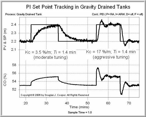
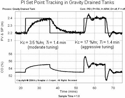
Again, the aggressive tuning values provide for a more active response.

Aside: it may appear that the random noise in the PV measurement signal is different in the two plots above, but it is indeed the same. Note that the span of the PV axis in each plot differs by a factor of four. The narrow span of the set point tracking plot greatly magnifies the signal traces, making the noise more visible.

Comparison With P-Only Control
The performance of a P-Only controller in addressing the same disturbance rejection and set point tracking challenge is shown here. A comparison of that study with the results presented here reveals that PI controllers:
▪ can eliminate the offset associated with P-Only control,
▪ have integral action that increases the tendency for the PV to roll (or oscillate),
▪ have two tuning parameters that interact, increasing the challenge to correct tuning when performance is not acceptable.

Derivative Action
The addition of the derivative term to complete the PID algorithm provides modest benefit yet significant challenges.

Return to the Table of Contents to learn more.