Quantifying Dynamic Process Behavior
Step 3 of the PID controller design and tuning recipe is to approximate process bump test data by fitting it with a first order plus dead time (FOPDT) dynamic model.
Data from a proper bump test is rich in dynamic information that is characteristic of our controller output (CO) to measured process variable (PV) relationship. A FOPDT model is a convenient way to quantify (assign numerical values to) key aspects of this CO to PV relationship for use in controller design and tuning.
In particular, when the CO changes:
▪ Process gain, Kp, describes the direction and how far the PV moves
▪ Time constant, Tp, describes how fast the PV responds
▪ Dead time, Өp, describes how much delay occurs before the PV first begins to move
In the investigation below, we isolate and study each FOPDT parameter individually to establish its contribution to the model response curve. By the end of the study, we (hopefully) will have established the power and utility of this model in describing a broad range of common process behaviors.
Aside: the FOPDT dynamic model is a linear, ordinary differential equation describing how PV(t) responds over time to changes in CO(t): 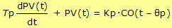 Where in this case study: t [=] min, PV(t) [=] °C, CO(t – Өp) [=] % Where in this case study: t [=] min, PV(t) [=] °C, CO(t – Өp) [=] % |
The Base Case Model
Each plot in this article shows the identical bump test data that was used in the jacketed stirred reactor study presented here. The CO step and PV response data are shown as black curves. The response of the computed FOPDT model is shown as a yellow curve.
The parameter values used to compute all of the FOPDT model responses are listed at the bottom of each plot. Throughout the study, the model parameter units are:
Kp [=] oC/%, Tp [=] min, Өp [=] min
The plot below shows a FOPDT model fit as computed by commercial software. We call this fit “good” or “descriptive” because we can visually see that the computed yellow model closely tracks the measured PV data.
If no significant disturbances occurred during the bump test to corrupt the response, then we can have confidence in our data set. And if the FOPDT model reasonably describes the data, as it does above, then a controller designed and tuned using the parameters from the model will perform as we expect. This, in fact, is the very reason we fit the model in the first place.
Kp is the “How Far” Variable
Process gain, Kp, describes the direction and how far the PV moves in response to a change in CO.
The direction is established with the sign of Kp. We recognize that in this case, Kp must be negative because when the CO moves in one direction, the PV moves in the other. We keep the negative sign throughout this study and focus on how the absolute size of Kp impacts model response behavior.
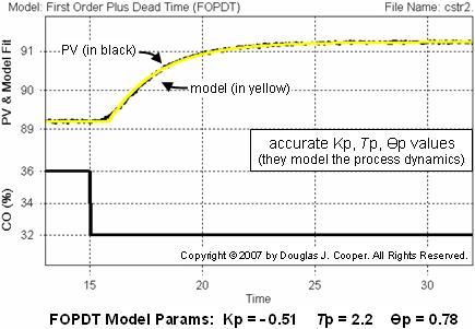
Below we compute and display the FOPDT model response using the base case time constant, Tp, and dead time, Өp. The yellow response curve below is different because the process gain used in the model has been increased in absolute size from the base case value of Kp = – 0.51 up to Kp = – 0.61.
With a larger model Kp, the “how far” response of the yellow curve clearly increases (more discussion on computing Kp here). Though perhaps not easy to see, the “how fast” and “how much delay” aspects of the response have not been impacted by the change in Kp.
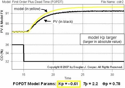
Below we compute the yellow FOPDT model response using the base case Tp and Өp, only this time, the process gain used in the model has been decreased from the base case Kp = – 0.51 down to Kp = – 0.41 (decreased in absolute size).
With a smaller Kp, we see that the computed model curve undershoots the PV data. We thus establish that process gain, Kp, dictates how far the PV travels in response to changes in CO.
Tp is the “How Fast” Variable
Process time constant, Tp, describes how fast the PV moves in response to changes in CO. The plot at the top of this article establishes that when Tp = 2.2, the speed of response of the model matches that displayed by the PV data.
Below we compute and display the FOPDT model response curve using the base case gain, Kp, and dead time, Өp. The curve is different because the time constant used to compute the yellow model response has been increased from the base case Tp = 2.2 up to Tp = 4.0.
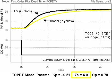
Recall that for step test data like that above, Tp is the time that passes from when the PV shows its first clear movement until when it reaches 63% of the total DPV change that is going to occur (more discussion on computing Tp here).
Since Tp marks the passage of time, a larger time constant describes a process that will take longer to complete its response. Put another way, a process with a larger Tp moves slower in response to changes in CO.
A very important observation in the above plot is that the yellow model curve, even though it moves more slowly than in the base case, ultimately reaches and levels out at the black PV data line. This is because the model response was generated using the base case Kp = – 0.51.
If we accept that the size of Kp alone dictates “how far” a response will travel, then this result is consistent with our understanding.
Below we show the yellow FOPDT model response using the base case Kp and Өp. The response curve is different because the model computation uses a process time constant that has been decreased from the base case Tp = 2.2 down to Tp = 1.0.
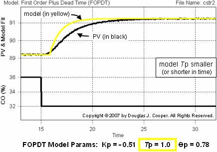
A smaller Tp means a process will take a shorter amount of time to complete its response. Thus, a process with a smaller time constant is one that moves faster in response to CO changes.
Again note that the yellow model response curve levels out at the black PV data line because the base case value of Kp = – 0.51 was used in computing “how far” the model response will travel.
Өp is the “With How Much Delay” Variable
If we examine all of the plots above we can observe that the “how much delay” behavior of the yellow model response curves are all the same, regardless of changes in Kp or Tp.
That is, the time delay that passes from when the CO step is made until when the model shows its first clear response to that action is the same regardless of the process gain and/or time constant values used (more discussion on computing Өp here).
This is because it is Өp alone that dictates the “how much delay” model response behavior.
To illustrate, below we compute and display the FOPDT model response curve using the base case process gain, Kp, and time constant, Tp. The yellow response is different in the plot below because the model dead time has been increased from the base case value of Өp = 0.78 up to Өp = 2.0.
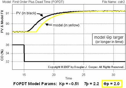
As the plot above shows, increasing dead time simply shifts the yellow model response curve without changing its shape in any fashion. A larger dead time means a longer delay before the response first begins.
The “how far” and “how fast” shape remains identical in the model response curve above because it is Kp and Tp that dictate these behaviors.
Below we show the yellow FOPDT model response using the base case Kp and Tp. The response curve is different because the model computation uses a dead time value that has been decreased from the base case Өp = 0.78 down to Өp = 0.
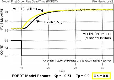
As shown in the plot above, if we specify no delay (i.e., Өp = 0), then the computed yellow model response curve starts to respond the instant that the CO step is made.
Conclusions
The above study illustrates that each parameter of the FOPDT model describes a unique characteristic of dynamic process behavior:
▪ Process gain, Kp, describes the direction and how far the PV moves.
▪ Time constant, Tp, describes how fast the PV responds.
▪ Dead time, Өp, describes how much delay occurs before the PV first begins to move.
Knowing how a PV will behave in response to a change in CO is fundamental to controller design and tuning.
For example, a controller must be tuned to make small corrective actions if every CO change causes a large PV response (if Kp is large). And if Kp is small, then the controller must be tuned to make large CO corrective actions whenever the PV starts to drift from set point.
If the time constant of a process is long (if a process responds slowly), then the controller must not be issuing new corrective actions in rapid fire. Rather, the controller must permit previous CO actions to show their impact before computing further actions.
We see exactly how the FOPDT model parameters are used as a basis for controller design and tuning in a host of articles in this e-book.