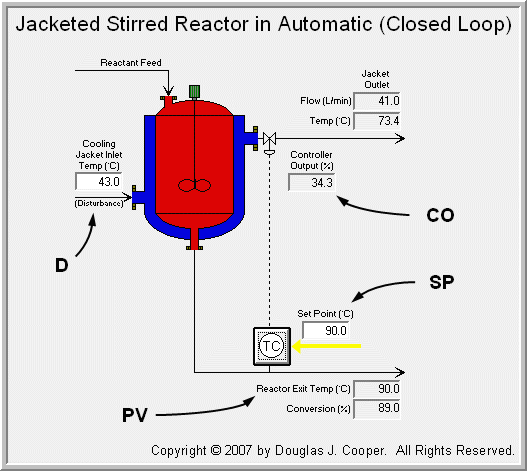
The control objective for the jacketed reactor is to minimize the impact on reactor operation when the temperature of the liquid entering the cooling jacket changes (detailed discussion here). As a base case study, we establish here the performance capabilities of a PI controller in achieving this objective.

    


The important variables for this study are labeled in the graphic (click for large view):
  CO = signal to valve that adjusts cooling jacket liquid flow rate (controller output, %)
  PV = reactor exit stream temperature (measured process variable, ^oC)
  SP = desired reactor exit stream temperature (set point, ^oC)
  D   = temperature of cooling liquid entering the jacket (major disturbance, ^oC)

We follow our industry proven recipe to design and tune our PI controller:

Step 1: Design Level of Operation (DLO)
The details of expected process operation and how this leads to our DLO are presented in this article and are summarized:
  ▪ Design PV and SP = 90 ^oC with approval for brief dynamic (bump) testing of ±2 ^oC.
  ▪ Design D = 43 ^oC with occasional spikes up to 50 ^oC.

Step 2: Collect Process Data around the DLO
When CO, PV and D are steady near the design level of operation, we bump the process as detailed here to generate CO-to-PV cause and effect response data.

Step 3: Fit a FOPDT Model to the Dynamic Process Data
We approximate the dynamic behavior of the process by fitting a first order plus dead time (FOPDT) dynamic model to the test data from step 2. The results of the modeling study are presented in detail here and are summarized:
  ▪ Process gain (direction and how far), Kp = – 0.5 ^oC/%
  ▪ Time constant (how fast), Tp = 2.2 min
  ▪ Dead time (how much delay), Өp = 0.8 min

Step 4: Use the FOPDT Parameters to Complete the Design
As in the heat exchanger PI control study, we explore what is often called the dependent, ideal form of the PI control algorithm:

  Where:
    CO = controller output signal (the wire out)
    CO_bias = controller bias or null value; set by bumpless transfer
    e(t) = current controller error, defined as SP – PV
    SP = set point
    PV = measured process variable (the wire in)
    Kc = controller gain, a tuning parameter
    Ti = reset time, a tuning parameter

Aside: our observations using the dependent ideal PI algorithm directly apply to the other popular PI controller forms. For example, the integral gain for the independent algorithm form, written as:      can be computed as:  Ki = Kc/Ti. The Kc is the same for both forms, though it is more commonly called the proportional gain for the independent algorithm.

• Sample Time, T
Best practice is to set the loop sample time, T, at one-tenth the time constant or faster (i.e., T ≤ 0.1Tp). Faster sampling may provide modestly improved performance, while slower sampling can lead to significantly degraded performance.

In this study, T ≤ 0.1(2.2 min), so T should be 13 seconds or less. We meet this with the sample time option available from most commercial vendors:
  ◊ sample time, T = 1 sec

• Control Action (Direct/Reverse)
The jacketed stirred reactor process has a negative Kp. That is, when CO increases, PV decreases in response. Since a controller must provide negative feedback, if the process is reverse acting, the controller must be direct acting. That is, when in automatic mode (closed loop), if the PV is too high, the controller must increase the CO to correct the error. Since the controller must move in the same direction as the problem, we specify:
  ◊ controller is direct acting

• Dead Time Issues
If dead time is greater than the process time constant (Өp > Tp), control becomes increasingly problematic and a Smith predictor can offer benefit. For this process, the dead time is smaller than the time constant, so:
  ◊ dead time is small and not a concern

• Computing Controller Error,  e(t)
Set point, SP, is manually entered into a controller. The measured PV comes from the sensor (our wire in). Since SP and PV are known values, then at every loop sample time, T, controller error can be directly computed as:
  ◊ error, e(t) = SP - PV

• Determining Bias Value, CO_bias
CO_bias is the value of CO that, in manual mode, causes the PV to steady at the DLO when the major disturbances are quiet and at their normal or expected values. When integral action is enabled, commercial controllers determine the bias value with a bumpless transfer procedure.

That is, when switching to automatic, the controller initializes the SP to the current value of PV, and CO_bias to the current value of CO. By choosing our current operation as our design state (at least temporarily at switchover), there is no corrective action needed by the controller that will bump the process. Thus,
  ◊ controller bias, CO_bias = current CO for a bumpless transfer

• Controller Gain, Kc, and Reset Time, Ti
We use our FOPDT model parameters in the industry-proven Internal Model Control (IMC) tuning correlations to compute PI tuning values.

The first step in using the IMC correlations is to compute Tc, the closed loop time constant. Tc describes how active our controller should be in responding to a set point change or in rejecting a disturbance.

The performance implications of choosing Tc have been explored previously for PI control of the heat exchanger and the gravity drained tanks case studies.

In short, the closed loop time constant, Tc, is computed based on whether we seek:
 ▪ aggressive action and can tolerate some overshoot and oscillation in the PV response,
 ▪ moderate action where the PV will move reasonably fast but show little overshoot,
 ▪ conservative action where the PV will move in the proper direction, but quite slowly.

Once this decision is made, we compute Tc with these rules:
 ▪ Aggressive Response:    Tc is the larger of  0.1·Tp  or 0.8·Өp
 ▪ Moderate Response:      Tc is the larger of    1·Tp  or    8·Өp
 ▪ Conservative Response: Tc is the larger of  10·Tp   or  80·Өp

With Tc computed, the PI controller gain, Kc, and reset time, Ti, are computed as:

Notice that reset time, Ti, is always equal to the process time constant, Tp, regardless of desired controller activity.

a) Moderate Response Tuning:
For a controller that will move the PV reasonably fast while producing little to no overshoot, choose:

Moderate Tc = the larger of 1·Tp or 8·Өp
                   = larger of 1(2.2 min) or 8(0.8 min)
                   = 6.4 min

Using this Tc and our model parameters in the tuning correlations above, we arrive at the moderate tuning values:

 

b) Aggressive Response Tuning:
For an active or quickly responding controller where we can tolerate some overshoot and oscillation as the PV settles out, specify:

Aggressive Tc = the larger of 0.1·Tp or 0.8·Өp
                    = larger of 0.1(2.2 min) or 0.8(0.8 min)
                    = 0.64 min

and the aggressive tuning values are:

 

Implement and Test
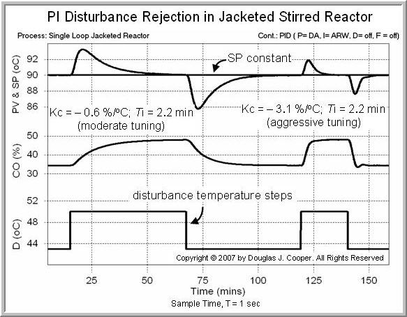
The ability of the PI controller to reject changes in the cooling jacket inlet temperature, D, is pictured below (click for a large view) for the moderate and aggressive tuning values computed above. Note that the set point remains constant at 90 ^oC throughout the study.

As expected, the aggressive controller shows a more energetic CO action, and thus, a more active PV response.

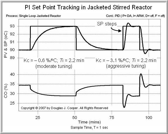
While not our design objective, presented below is the set point tracking ability of the PI controller (click for a large view) when the disturbance temperature is held constant.

The plot shows that set point tracking performance matches the descriptions used above for choosing Tc:

▪	Use aggressive action if we seek a fast response and can tolerate some overshoot and oscillation in the PV response.
▪	Use moderate action if we seek a reasonably fast response but seek little to no overshoot in the PV response.

Important => Ti Always Equals Tp
As stated above, the rules provide a constant reset time, Ti, regardless of our desired performance. So if we believe we have collected a good process data set, and the FOPDT model fit looks like a reasonable approximation of this data, then we have a good estimate of the process time constant and Ti = Tp regardless of desired performance.

If we are going to tweak the tuning, Kc should be the only value we adjust. For example, if we seek a performance between moderate and aggressive, we average the Kc values while Ti remains constant.

Return to the Table of Contents to learn more.

Copyright © 2008 by Douglas J. Cooper. All Rights Reserved.