By Bob Rice1 and Doug Cooper
The control objective for the pumped tank process is to maintain liquid level at set point by adjusting the discharge flow rate out of the bottom of the tank. This process displays the distinctive integrating (or non-self regulating) behavior, and as such, presents an interesting control challenge.
The process graphic below (click for a large view) shows the pumped tank in automatic mode (also called closed loop):
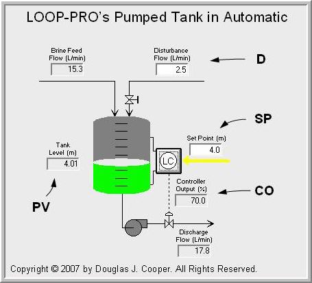
The important variables for this study are labeled in the above graphic:
CO = signal to valve that adjusts discharge flow rate of liquid (controller output, %)
PV = measured liquid level signal from the tank (measured process variable, m)
SP = desired liquid level in tank (set point, m)
D = flow rate of liquid entering top of tank (major disturbance, L/min)
We follow the controller design and tuning recipe for integrating processes in this study as we design and test a PI controller. Please recall that there are subtle yet important differences between this procedure and the design and tuning recipe used for the more common self regulating process.
Step 1: Design Level of Operation (DLO)
We choose the DLO to be the same as that used in this article so we can build upon our previous modeling efforts:
▪ design value for PV and SP = 4.8 m
▪ design value for D = 2.5 L/min
Characteristic of real integrating processes, the pumped tank PV does not naturally settle at a steady operating level if CO is held constant. This lack of a natural “balance point” means we will not specify a CO as part of our DLO.
Step 2: Collect Process Data around the DLO
When PV and D are near the design level of operation and D is substantially quiet, we perform a dynamic test and generate CO-to-PV cause and effect dynamic data.
Because the PV of integrating processes tends to drift in manual mode (open loop), one alternative is to perform an open loop dynamic test that does not require bringing the process to steady state. As detailed in this article, the procedure is to maintain CO at a constant value until a slope trend in the PV can be visually identified. We then move the CO to a different value and hold it until a second PV slope is established. The article shows how to analyze the resulting plot data with hand calculations to obtain the FOPDT Integrating model for step 3 of the design and tuning recipe.
An alternative approach, presented below, is to use automatic mode data. When in closed loop, dynamic data is generated by bumping the SP. For model fitting purposes, the controller must be tuned such that the CO takes clear and sudden actions in response to the SP changes, and these must force PV movements that dominate the measurement noise.
Because a closed loop approach makes it possible to generate integrating process dynamic test data that begins at steady state, we can use model fitting software much like we did in this closed-loop set point driven study.
Below (click for a large view) we see the pumped tank process under P-Only control. As shown in the left half of the plot, while the major disturbance is quiet and at its design level, we are able to obtain good set point tracking performance with P-Only control.
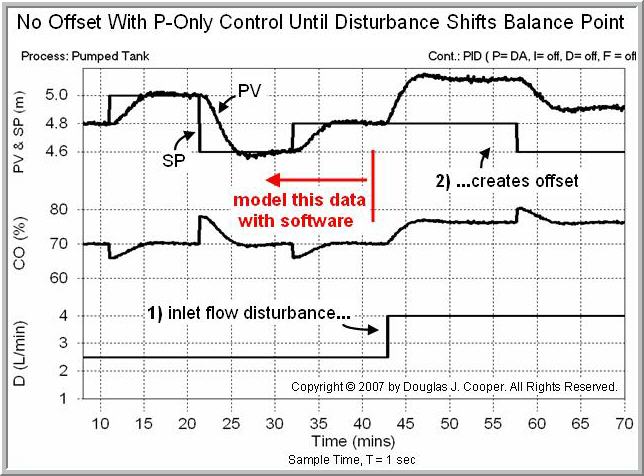
As we discuss here and as shown above, a P-Only controller is able to provide good SP tracking performance with no offset as long the major disturbances are quiet and at their design values. Industrial processes can have many disturbances that impact operation. If any one of them changes, as happens in the above plot at roughly 43 minutes, then the simple P-Only controller is incapable of eliminating what becomes a sustained offset (i.e., incapable of making e(t) = SP – PV = 0)
This is why the integral action of a PI controller offers value even though the process itself possesses a naturally integrating behavior.
Note: in a surge tank where exit flow smoothing is more important than maintaining the measured level at SP, offset may not be considered a problem to be solved. Each situation must be considered on its own merits.
The red label in the above plot indicates that the left half contains dynamic response data that begins at steady state and that is not corrupted by disturbance changes. We isolate this data and model it as described in step 3 below.
Step 3: Fit a FOPDT Integrating Model to the Dynamic Process Data
We obtain an approximating description of the closed loop CO to PV dynamic behavior by fitting the process data with a first order plus dead time integrating (FOPDT Integrating) model of the form:
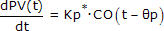
where
Kp* = integrator gain, with units [=] PV/(CO·time)
Өp = dead time, with units [=] time
Cropping the data and fitting the FOPDT Integrator model takes but a few mouse clicks with a commercial software tool (recall that an alternative graphical hand calculation method is described here).
The results of the automated model fit are shown below (click for a large view). The visual similarity between the model and data gives us confidence that we have a meaningful description of the dynamic behavior of this process. The Kp* and Өp for this approximating model are shown at the bottom of the plot.
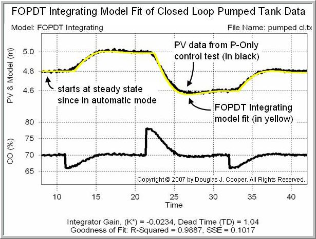
The model fitting software performs a systematic search for the combination of model parameters that minimizes the sum of squared errors (SSE), computed as:
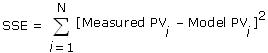
The Measured PV is the actual data collected from our process. The Model PV is computed using the model parameters from the search routine and the actual CO data from the file. N is the total number of samples in the file. In general, the smaller the SSE, the better the model describes the data.
The table below summarizes the model parameters from the above closed loop model fit as well as the results from the open loop slope driven analysis detailed in this article.
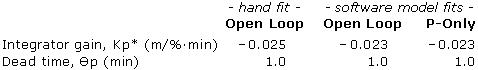
For the control studies in step 4, we will use:
▪ Kp* = – 0.023 m/%·min
▪ Өp = 1.0 min
Step 4: Use the FOPDT Integrating Parameters to Complete the Design
• Sample Time, T
The design and tuning recipe for integrating processes suggests setting the loop sample time, T, at one-tenth the process dead time or faster (i.e., T ≤ 0.1Өp). Faster sampling provides equally good, but not better, performance.
In this study, T ≤ 0.1(1.0 min), so T should be 6 seconds or less. We meet this with the sample time option available from virtually all commercial vendors:
◊ sample time, T = 1 sec
• Control Action (Direct/Reverse)
The pumped tank has a negative Kp*, so when CO increases, PV decreases in response. Since a controller must provide negative feedback, if the process is reverse acting, the controller must be direct acting. Thus, if the PV is too high, the controller must increase the CO to correct the error. Since the controller moves in the same direction as the problem, we specify:
◊ controller is direct acting
• Computing Controller Error, e(t)
Set point, SP, is manually entered into a controller. The measured PV comes from the sensor (our wire in). Since SP and PV are known values, then at every loop sample time, T, controller error can be directly computed as:
◊ error, e(t) = SP – PV
• Determining Bias Value, CObias
The lack of a natural balance point with integrating processes makes the determination of a design CObias problematic. The solution is to use bumpless transfer. That is, when switching to automatic, initialize SP to the current value of PV and CObias to the current value of CO (most commercial controllers are already programmed this way). By choosing our current operation as our design state at switchover, there is no corrective actions needed by the controller and it can smoothly engage, thus:
◊ controller bias, CObias = CO that exists at switch over
• Controller Gain, Kc, and Reset Time, Ti
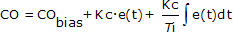
We use our FOPDT Integrating model parameters in the industry-proven Internal Model Control (IMC) tuning correlations to compute PI tuning values. Though all PI forms are equally capable, we use the dependent, ideal form of the PI algorithm in this study:
The first step in using the IMC correlations is to compute Tc, the closed loop time constant. Tc describes how active our controller should be in responding to a set point change or in rejecting a disturbance. For integrating processes, the design and tuning recipe suggests:
Tc = 3Өp = 3(1.0 min) = 3 min
With Tc computed, the PI controller gain, Kc, and reset time, Ti, are computed as:
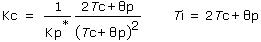
Substituting the Kp*, Өp and Tc identified above into these tuning correlations, we compute:
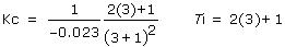
or
▪ Kc = – 19 m/%
▪ Ti = 7 min
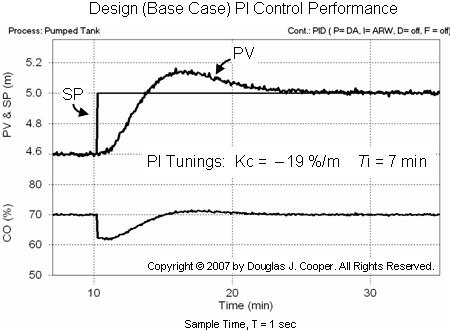
Below is the performance of this PI controller (with Kc = – 19 and Ti = 7) on the pumped tank (click for a large view). The plot includes the same set point tracking and disturbance rejection test conditions as were used in the P-Only controller plot near the top of this article.

As labeled in the plot, our PI control set point response now includes some overshoot. Recall that the P-Only controller, shown near the top of this article, can provide a rapid set point response with no overshoot, that is, until a disturbance changes the balance point of the process.
The benefit of integral action is that when a disturbance occurs, a PI controller can reject the upset and return the PV to set point. This is because the constant summing ofintegral action continues to move the CO until controller error is driven to zero.
Thus, PI control requires that we accept some overshoot during set point tracking in exchange for the ability to reject disturbances. In many industrial applications, this is considered a fair trade.
Tuning Sensitivity Study
Below is the set point tracking performance of our PI controller on the pumped tank. The controller tuning (Kc = – 19 m/%, Ti = 7 min) is determined as detailed in the step-by-step recipe above.
Some questions to consider are:
▪ How does performance vary as the tuning values change?
▪ How can we avoid overshoot if we find such behavior undesirable?
Below (click for a large view) is a tuning map for a PI controller implemented on the pumped tank integrating process. The center plot is the identical base case performance plot shown above.
The complete map shows set point tracking performance when controller gain (Kc) and reset time (Ti) are individually doubled and halved.

While “good” or “best” performance is a matter best decided by the operations staff, the above map makes it clear that our recipe does an excellent job of meeting the desire for a reasonably rapid rise, a modest overshoot and a quick settling time.
Unfortunately, eliminating overshoot altogether does not appear to be one of our options for PI control of integrating processes.
Final Thoughts
The design and tuning recipe for integrating processes provides the above base case performance with minimal testing on our process. In a manufacturing environment where we need a fast solution with minimal disruption, this recipe is certainly one to have in our tool box.
_______
1. Bob Rice holds primary responsibility at Control Station for training and software development, deployment, and support. Dr. Rice has published extensively on topics associated with automatic process control, including non-self-regulating processes and model predictive control. Prior to joining Control Station, Dr. Rice held engineering and technical positions with PPG Industries and The Walt Disney Company.
Robert Rice, Ph.D.
Director of Solutions Engineering
Control Station, Inc.
One Technology Drive
Tolland, CT 06084
Phone: (860) 872-2920
Email: bob.rice@controlstation.com
Web: http://www.controlstation.com