By Fred Thomasson1
In the Control Magazine article entitled Envelope Optimization by Bela Liptak (www.controlglobal.com; 1998), a multivariable control strategy is described whereby a process is “herded” to stay within a safe operating envelope while the optimization proceeds.
Building on that work, a method to implement Envelope Optimization using fuzzy logic is described in this article (a primer on fuzzy logic and fuzzy control can be found here).
When some of us think about optimization, we think about complex gradient search methods. This is something that a PhD dreams up but they rarely ever work in the plant. After the theoretician goes back to the R & D facility, the plant engineers are charged with keeping it running. After a few glitches that nobody understands, it is turned off and that marks the end of the optimization effort.
Background
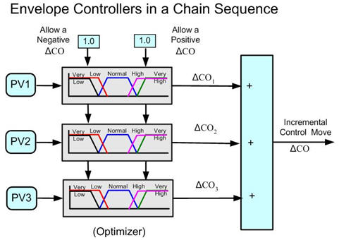
The basic building tool for this optimization methodology is the fuzzy logic Envelope Controller (EC) function block. Such EC blocks are often chained (or sequenced) one after the other. As shown below, each EC in the chain sequence focuses on a single process variable, with the complete chain forming an efficient and sophisticated optimization strategy.
With such a chain sequence construction, it is possible to incorporate many constraints. It is not difficult to add or remove a constraint or change its priority, even in real time.
To better understand the operation of the chain sequence shown in the figure above, use the following analogy. Three operators are sitting side by side in front of their own operator’s console. Each operator can only view a single PV. There are operating constraints for the PV [Very Low, Low, Normal, High, Very High]. Each operator can make incremental control moves to the single output variable. They can make a move once a minute.
Operator #1 monitors PV1. If PV1 is Very High, a fixed size negative incremental move will be made. If PV1 is Very Low, a positive move will be made. Otherwise no control move is made. Control moves are made to insure the constraints are not exceeded.
Operator #2 monitors PV2. If PV2 is Very High, a fixed size negative incremental move needs to be made. If PV2 is Very Low, a positive move needs to be made. Otherwise no control move needs to be made. But first, permission from Operator #1 is required. If PV1 is Very High, a positive control move is not allowed. If PV1 is Very Low, a negative move is not allowed. Otherwise permission is granted for any move.
Permission is a fuzzy variable which varies from 0.0 to 1.0. Permission of 0.50 allows Operator # 2 to make half of the fixed control move.
Operator #3 monitors PV3. This operator performs the optimization function. In this example, it will be to maximize production rate. Therefore PV3 is the production rate. If PV3 is not High, a positive control move will be made. This operator only makes positive control moves. But first permission from both Operator #1 and Operator #2 is required. It will insure that the constraints are not violated. This requires that neither PV1 or PV2 are High. Operator #3 will stop making control moves when PV3 becomes High.
It is up to Operator #1 and Operator #2 to reduce the production rate if a constraint is exceeded.
A detailed description of the Envelope Controller block is given in the next section. However it may be clearer to go directly to the two optimization examples at the end of the article and then come back and read the rest of the article. The description of the Envelope Controller Block is included for completeness.
Two optimization examples are shown later in this article. The first deals with minimizing the amount of combustion air for an industrial power boiler. The second deals with minimizing the outlet pressure of a forced draft fan of an industrial power boiler to minimize energy losses.
This controller is best suited to applications where there are multiple measured input variables that must stay within prescribed limits and there is a single output variable.
The Envelope Controller Block
Before discussing how the fuzzy logic Envelope Controller (EC) function block can be chained in a sequence to form an optimization strategy, we first consider the function of a single EC block.
A schematic of the basic EC block is shown in the figure below (click for a large view):
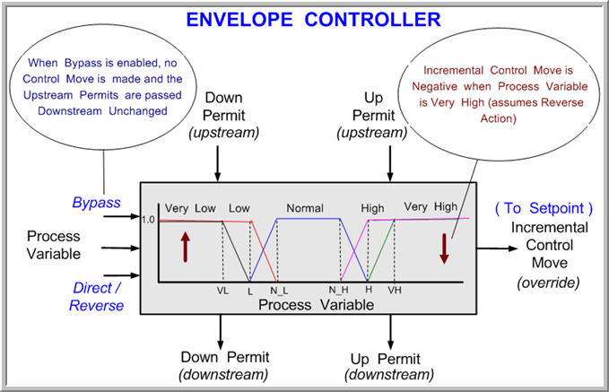
As will be illustrated in the examples later in this article, the terms “upstream” and “downstream” refer to the flow of information in the chain sequence of EC’s in the optimization strategy and not the flow of material through processing units.
The basic construction is to use the chain of ECs to oversee constraints in order of priority. The last EC in the chain is used as an optimizer.
Envelope Controller Inputs, Outputs and Parameters:
Inputs:
1. Process Variable (continuous PV)
2. Down_Permit (0 – 1.0)
3. Up_Permit (0 – 1.0)
Outputs:
1. Incremental Control Output (continuous CO)
2. Down_Permit (0 – 1.0)
3. Up_Permit (0 – 1.0)
Parameters to Specify:
1. NEG – (size of negative move)
2. POS – (size of positive move)
3. Six breakpoints (VL, L, N_L, N_H, H, VH) on the PV axis which uniquely identifies all five membership functions
4. G – (Overall Gain)
Switches to Set:
1. Bypass (on/off)
2. Control Action (Reverse or Direct)
Membership Functions:
Five membership functions are shown superimposed in the Envelope Controller (EC) figure above. Each membership function is a fuzzifier. A continuous process variable (PV) is mapped to 5 sets of fuzzy variables whose values are between 0.0 and 1.0. They are:
| 1. | PV_VL = μ1(PV) | VL: Very Low |
| 2. | PV_L = μ2(PV) | L: Low |
| 3. | PV_N = μ3(PV) | N: Normal |
| 4. | PV_H = μ4(PV) | H: High |
| 5. | PV_VH = μ5(PV) | VH: Very High |
Where μ means degree of membership. When PV is midway between VL and L in the above EC diagram, for example, then μ1 = 0.5 and μ2 = 1.0. All the rest are 0.0.
The fuzzy variables, such as PV_N, are called linguistic variables. Here, PV_N means “PV is Normal.” Similarly, PV_VH means “PV is very high.”
Control Action Switch
This switch has two positions as shown in the figure above: “Reverse” and “Direct.” In most processes, when the process variable (PV) exceeds the high limit, the controller output (CO) must be decreased to bring it back into the safe operating envelope. The control action switch must be in the “Reverse” position for this to occur.
However, there are processes where the CO must be increased to bring it back into the safe operating envelope if the PV exceeds the high limit. The position of the control action switch must be “Direct” for these processes.
Thus, the control action switch of the EC is analogous to the direct and reverse action of PID controllers.
Bypass Selector Switch
As shown in the figure above, an EC has a bypass switch. When the EC is in bypass mode, the EC is switched out of the chain sequence and the Up Permit_In and Down Permit_In signals pass through the EC unchanged as if it does not exist.
Controller Functionality
The membership functions of each EC define the safe operating region for the incoming PV. When the PV is in the “PV Normal Region,” the incremental control move (override) produced by the EC is 0.0. The Up Permit_In and Down Permit_In values are passed unmodified to the next Envelope Controller in the chain sequence.
To simplify the discussion, we assume the EC uses reverse action in the following logic. A direct action EC uses analogous, though opposite, logic.
When the PV entering an EC is in the “High” or “Low” regions, the Up Permit_Out or the Down Permit_Out variable is modified by the fuzzy variable Correction Factors (CF):
1. Up Permit_CF = NOT (H)
2. Down Permit_CF = NOT (L) where NOT (x) = 1–x
The product operator (μA[PV]*μB[PV]) is used in the EC computation. This is one version of the fuzzy “AND.” The Up Permit_In and Down Permit_In are multiplied by the appropriate correction factors to become:
1. Up Permit_Out = (Up Permit_In)* (Up Permit_CF )
2. Down Permit_Out = (Down Permit_In)*( Down Permit_CF)
When the PV enters the “Very High” or “Very Low” regions, an incremental control move (override) is made to nudge the PV back into the safe region:
1. ΔCO = (Down Permit_In)*(PV_VH)*NEG*G
2. ΔCO = (Up Permit_In)*(PV_VL)*POS*G
This is a simple two-rule controller. For a EC with reverse action, these rules can be summarized:
[R1] if there is permission to make a negative control move and the PV is very
high (VH), then make a negative incremental control move.
[R2] if there is permission to make a positive control move and the PV is very
low (VL), then make a positive incremental control move.
NEG*G and POS*G are singletons. ΔCO is the defuzzified value. It is simply the product of the singleton and the truth of the rule. There are many defuzzification techniques. A simple but highly effective method uses singletons and a simple center of gravity calculation. This is the one used in these applications.
Chaining in Sequence
ECs are chained in sequence to form an efficient Envelope Optimization controller. With a proper number of constraints in proper priority order, they form a safe operating envelope for the process. ECs can be implemented in many modern process control system to create Envelope Optimization logic.
· Example: Minimum Excess Air Optimization
This application of Envelope Optimization is for an industrial power boiler. As shown below (click for a large view), it uses five ECs chained in sequence. Like many optimization problems, the solution for minimum excess air optimization is found on the constraint boundary.

Control Objectives
1) Maintain combustion air at minimum flow required for safe operation and maximum boiler efficiency.
2) Stay within the safe operating envelope as defined by the limits of the first four ECs.
3) Take immediate corrective action when any of the prioritized constraints are violated.
4) Optimization must proceed slowly to avoid upsetting the process.
Optimization Functionality
The air-to-fuel (A/F) ratio is slowly reduced by the negative incremental moves made by the Optimizer EC (the last in the chain sequence) until a limit is reached on one of the first four ECs. This limit condition would then reduce the Down Permit entering the Optimizer EC to 0.0.
Notice that the Up and Down Permits are set to 1.0 at the top of the chain. If the PVs of the first four ECs are all in the “Normal” regions. The Up Permit and Down Permit will pass down the chain unmodified as 1.0.
The first EC sets the high and low limits for the A/F ratio. Note that this EC has the highest priority. If the A/F reaches its low limit, the Down Permit goes to 0.0. The second EC sets the high limit for Opacity (no low limit). The third EC sets the high and low limits for O2. The fourth EC sets the high limit for combustibles (unburned hydrocarbons). There is no low limit. Normally this control operates at the low limit for A/F ratio with low O2 and very low combustibles.
Aside: The optimization function is automatically disabled when the combustibles meter goes into self-calibration and resumes normal operation when the calibration is finished. The operator can also turn the optimization “off” at any time. The Minimum Excess Air Optimization can function with just O2 if the combustibles meter is out of service. The Combustibles EC would need to be placed on “bypass” for this to occur.
While the optimizing function is slow, that is not the case for the constraint override action. For example, if the O2 fell below the low limit, the A/F ratio would quickly increase to bring O2 back within the “Normal” region.
Tuning this control is not simple. It requires selecting numerous gains and membership breakpoints. The slope of the membership functions are part of the loop gain when override action is taking place.
While tuning the control is difficult, the good news is that once it is tuned it does not seem to require any tweaking afterwards. This particular application has used the same tuning parameters since it was commissioned several years ago with no apparent degradation in performance.
· Example: Forced Draft Fan Outlet Pressure Optimization
This application of Envelope Optimization is for an industrial power boiler. It uses five ECs chained together as shown in the graphic below (click for a large view).
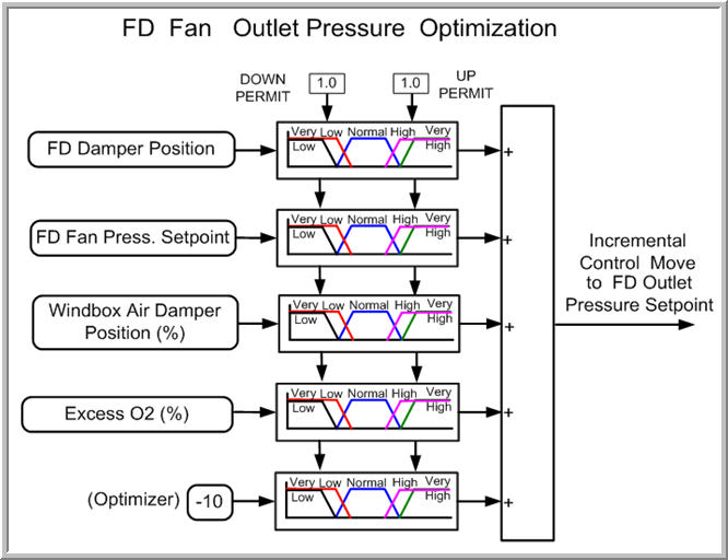
On this power boiler, the Forced Draft (FD) Fan Outlet Pressure is controlled with a PID controller. The PID controller accomplishes this by adjusting the inlet vanes. This provides a constant pressure source for the windbox air dampers. At high steaming rates the pressure needs to be fairly high (about 10.0 inches). At lower steaming rates it doesn’t need to be this high and results in a large pressure drop across the windbox dampers. This results in more energy being used than is necessary.
Control Objectives
1) Maintain the FD fan outlet pressure at the minimum pressure required to provide the amount of air needed for combustion.
2) Maintain the windbox air dampers in a mid-range position for maximum controllability.
3) Stay within the “Safe Operating Envelope” as defined by the limits of the first four Envelope Controllers.
Optimization Functionality
The FD fan outlet pressure set point is slowly reduced by negative incremental moves made by the last Envelope Controller (Optimizer) until a limit is reached on one of the first four ECs. Normally it is the FD Fan Pressure set point EC that reaches its low limit and reduces the Down Permit to 0.0 entering the Optimizer EC.
The Down Permit does not suddenly go to 0.0 as the low limit is reached. It gradually decreases because of the slope of the PV_L membership function. When the truth of PV_L is 0.5, the Down Permit becomes 0.5 and only half of the Optimizer’s regular incremental move is made. Likewise, when PV_L is 0.1 only one tenth of the Optimizer’s regular move is made.
The first EC sets the high and low limits for the FD damper position. The actuator always has the highest priority. The second EC sets the high and low limits for the FD outlet pressure set point. The third EC sets the high limit for the windbox air dampers (no low limit). The fourth EC sets the low limit for O2 (no high limit).
At low boiler steaming rates the FD fan outlet pressure is held at minimum by the second EC. As the boiler steaming rate increases, the windbox dampers open further to provide more combustion air. The damper position reaches its very high limit causing a positive incremental override control move from the third EC. This causes the pressure set point to increase. As the FD fan outlet pressure rises, the damper moves back to a lower value.
Note that the total incremental control move is made up of the sum of the moves from all of the ECs. In this situation, the new equilibrium occurs when the sum of the third and fifth ECs equal 0.0. The third EC is making a positive move and the Optimizer EC is making a negative move. If the gains and slopes of the membership functions of the third EC are not carefully selected, cycling (otherwise known as instability) will occur. In control jargon this feature could be called mid-ranging. It is desired to always have the windbox damper operating in its normal range.
If for some reason the O2 goes below its very low limit, positive incremental override control moves will be made by the fourth EC raising the FD fan outlet pressure. This increases air flow to the windbox. This is a safety feature.
Tuning this control is not simple. This is particularly true for the interaction between the third EC and the Optimizer. In this application none of the PVs have significant time constants or delays. Therefore predicted PVs were not used. While tuning the control is difficult, the good news is that once it is tuned it does not seem to require any tweaking afterwards. This particular application has used the same tuning parameters since it was commissioned several years ago with no apparent degradation in performance.
Final Thoughts
An interesting method to implement Envelope Optimization using fuzzy logic has been presented in this article. Constraints can be prioritized with those affecting safety and environmental concerns at the top of the list. The Envelope Controller is at the heart of the approach. Linking these controllers together in a chain allows one to form a “Safe Operating Envelope” which is the constraint boundary. Optimization proceeds as the process is kept within this envelope. Two examples were shown that use this methodology.
The reader should study some of the fundamental concepts of fuzzy logic if they are interested in an in-depth understanding of this approach. Understanding how to tune these controls is the most difficult part of the application. This can only be done during the startup phase or with a dynamic simulation.
The method described and the examples presented are valid for situations where there is only one variable to manipulate. This approach can be extended to problems where there are multiple variables to manipulate. The author has worked on problems where two variables were manipulated. It usually requires a sophisticated predictive model to provide inputs to some of the Envelope Controllers. It actually becomes a type of Model Predictive Control (MPC).
_______
1. About the Author
Fred Thomasson has worked as a process control engineer with a pulp and paper company for about 30 years. He has a PhD from the University of Virginia and has been very active in in the process control division of TAPPI, the leading association for the worldwide pulp, paper and packaging industries. He has a long-held interest in applying advanced control technology to process control and started using fuzzy logic control about 15 years ago. This article describes two actual applications that he implemented about six years ago, and they are still performing well today.
Fred Thomasson
55 Riverbend Road
Richmond Hill, GA 31324
Email: fthomasson@comcast.net