The control objective for the jacketed stirred reactor process is to minimize the impact on reactor operation when the temperature of the liquid entering the cooling jacket changes. We have previously established the performance capabilities of a PI controller in rejecting the impact of this disturbance.

Here we explore the performance of a PID with controller output (CO) filter algorithm in meeting this same disturbance rejection objective. We use the unified PID with CO filter controller in this study. As detailed in a prior article, the unified form is identical to a PID with external first-order CO filter implementation. Thus, the methods and observations from this investigation apply equally to both controller architectures.

The important variables for the jacketed reactor are (view a process graphic):
  CO = signal to valve that adjusts cooling jacket liquid flow rate (controller output, %)
  PV = reactor exit stream temperature (measured process variable, ^oC)
  SP = desired reactor exit stream temperature (set point, ^oC)
  D   = temperature of cooling liquid entering the jacket (major disturbance, ^oC)

We follow our industry proven recipe to design and tune our PID with CO filter controller. Recall that steps 1-3 of a design remain the same regardless of the controller used. For this process and objective, the results of steps 1-3 are summarized from previous investigations:

Step 1: Design Level of Operation (DLO)
DLO details are presented in this article and are summarized:
  ▪ Design PV and SP = 90 ^oC with approval for brief dynamic (bump) testing of ±2 ^oC
  ▪ Design D = 43 ^oC with occasional spikes up to 50 ^oC

Step 2: Collect Process Data around the DLO
When CO, PV and D are steady near the design level of operation, we bump the jacketed stirred reactor to generate CO-to-PV cause and effect process response data.

Step 3: Fit a FOPDT Model to the Dynamic Process Data
We approximate the dynamic behavior of the process by fitting a first order plus dead time (FOPDT) dynamic model to the test data from step 2. The results of the modeling study are summarized:
  ▪ process gain (direction and how far), Kp = – 0.5 ^oC/%
  ▪ time constant (how fast), Tp = 2.2 min
  ▪ dead time (how much delay), Өp = 0.8 min

Step 4: Use the FOPDT Parameters to Complete the Design

• Algorithm Form
A PID with CO filter controller, regardless of whether the filter is internal or external, presents us with a "four adjustable tuning parameter" challenge. As more parameters are included in our controller, the array of vendor algorithm forms increases.

The various controller forms are all capable of delivering a similar, predictable performance, as long as we match our algorithm with its proper tuning correlations. Certainly, a "guess and test" approach to tuning a four-mode controller while our process is making product is a sure path to wasting feedstock and utilities, creating safety and environmental concerns, and putting plant profitability at risk.

Modern loop tuning software will not only guide data analysis and model fitting, but will ensure our tuning matches our vendor's algorithm. Such software will even display expected final performance prior to implementation. If our task list includes maintaining and tuning control loops during production, such software will pay for itself in days.

• Sample Time
As discussed here, best practice is to set loop sample time to T ≤ 0.1Tp (10 times per time constant or faster). We meet this design criterion with the widely-available vendor option of T = 1.0 sec.

• Controller Action
Kp, and thus Kc, are negative for our jacketed stirred reactor process. Most commercial controllers have us specify a negative Kc by entering a positive value into the controller and then choosing the "direct acting" option (more discussion in this article). If the wrong control action is entered, the controller will drive the final control element to full on/open or full off/closed and remain there until a proper control action entry is made.

• Specify Desired Performance
We use the industry-proven Internal Model Control (IMC) tuning correlations in this study. IMC correlations employ a closed loop time constant, Tc, that describes the desired speed or quickness of our controller in responding to a set point change or rejecting a disturbance.

Our PI control study describes what to expect from an aggressive, moderate or conservative controller. Once our desired performance is chosen, the closed loop time constant is computed:
   ▪ aggressive performance:     Tc is the larger of  0.1·Tp or  0.8·Өp
   ▪ moderate performance:      Tc is the larger of     1·Tp or    8·Өp
   ▪ conservative performance:  Tc is the larger of   10·Tp or  80·Өp

• The Tuning Correlations
A previous article presents details of how to combine an external first-order filter into the unified ideal PID with internal filter form:

If our vendor offers the option, the preferred algorithm in industrial practice is PID with derivative on measurement, PV:

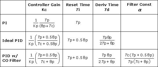
The IMC tuning correlations for either of the above PID with CO filter forms are the same and listed in the chart below. The chart also lists the tuning correlations as discussed in previous articles for the PI controller and ideal PID controller forms:

PID With CO Filter Disturbance Rejection Study
In the plots below, we compare the performance of the PID with CO filter controller side-be-side with that of the PI controller and the ideal (unfiltered) PID controller.

Our objective is rejecting the the impact on reactor operation when the temperature of cooling liquid entering the reactor jacket changes. We test both moderate and aggressive response tuning for the three controllers.

• Implement and Test
A comparison of the three controllers in rejecting a disturbance change in the cooling jacket inlet temperature, D, is shown below (click for a large view). This plot shows controller performance when using the moderate tuning values computed above. Note that the set point remains constant at 90 ^oC throughout the study.

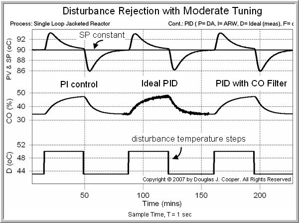
The PI controller performance is shown to the left in the plot above. The ideal PID performance is in the middle. The plot reveals that the benefit of derivative action is marginal at best. There is a clear penalty, however, in that derivative action causes the modest noise in the PV signal to be amplified and reflected as "chatter" in the CO signal.

To the right in the plot above is the performance of the PID with CO filter controller. The filter is effective in reducing the controller output chatter caused by the derivative action without degrading performance. In truth, however, the four tuning parameter PID with filter performs similar to the two tuning parameter PI controller.

The disturbance rejection performance of the controllers when tuned for aggressive action is shown below (click for a large view). Note that the axis scales for the plots both above and below are the same to permit a visual comparison.

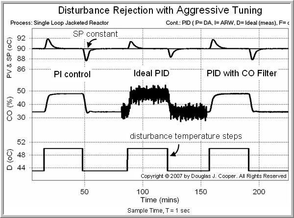
The aggressive tuning provides a smaller maximum deviation from set point and a faster settling time relative to the moderate tuning performance. The only obvious difference is that as a PID controller (middle of plot) becomes more aggressive in its actions, the CO chatter grows as a problem and filtering solutions become increasingly beneficial.

But ultimately, just as with the moderate tuning case, the two mode (or two tuning parameter) PI controller compares favorably with the four mode PID with CO filter controller.

While not our design objective, presented below (click for a large view) is the set point tracking ability of the aggressively tuned controllers when the disturbance temperature is held constant:

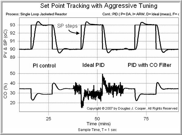
The set point tracking response of the ideal PID controller is marginally better in that it shows a slightly shorter rise time, smaller overshoot and faster settling time. The CO chatter that comes as a price for these minor benefits will likely increase maintenance costs as our final control element (e.g., valve, pump or compressor) wears from this excessive activity.

The four mode PID with CO filter addresses the chatter, but it is not clear that the added complexity is worth the marginal performance benefits.

Thus, many practitioners conclude that the PI controller provides the best balance of complexity and performance. It is faster to implement, easier to maintain, and provides performance approaching that of the PID with CO filter controller.

Return to the Table of Contents to learn more.

Copyright © 2007 by Douglas J. Cooper. All Rights Reserved.