The Cascade Control Architecture - Practical Process Control by Control Guru

The Cascade Control Architecture

Two popular control strategies for improved disturbance rejection performance are cascade control and feed forward with feedback trim.

Improved performance comes at a price. Both strategies require that additional instrumentation be purchased, installed and maintained. Both also require additional engineering time for strategy design, tuning and implementation.

The cascade architecture offers alluring additional benefits such as the ability to address multiple disturbances to our process and to improve set point response performance.

In contrast, the feed forward with feedback trim architecture is designed to address a single measured disturbance and does not impact set point response performance in any fashion (explored in a future article).

The Inner Secondary Loop
The dashed line in the block diagram below (click for a large view) circles a feedback control loop like we have discussed in dozens of articles on controlguru.com. The only difference is that the words "inner secondary" have been added to the block descriptions. The variable labels also have a "2" after them.

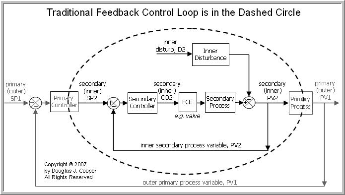
So,
SP2 = inner secondary set point
CO2 = inner secondary controller output signal
PV2 = inner secondary measured process variable signal

And
D2 = inner disturbance variable (often not measured or available as a signal)
FCE = final control element such as a valve, variable speed pump or compressor, etc.

The Nested Cascade Architecture
To construct a cascade architecture, we literally nest the secondary control loop inside a primary loop as shown in the block diagram below (click for a large view).

Note that outer primary PV1 is our process variable of interest in this implementation. PV1 is the variable we would be measuring and controlling if we had chosen a traditional single loop architecture instead of a cascade.

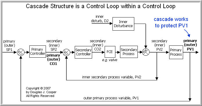
Because we are willing to invest the additional effort and expense to improve the performance response of PV1, it is reasonable to assume that it is a variable important to process safety and/or profitability. Otherwise, it does not make sense to add the complexity of a cascade structure.

Naming Conventions
Like many things in the PID control world, vendor documentation is not consistent. The most common naming conventions we see for cascade (also called nested) loops are:
▪ secondary and primary
▪ inner and outer
▪ slave and master
In an attempt at clarity, we are somewhat repetitive in this article by using labels like "inner secondary" and "outer primary."

Two PVs, Two Controllers, One Valve
Notice from the block diagrams that the cascade architecture has:
▪ two controllers (an inner secondary and outer primary controller)
▪ two measured process variable sensors (an inner PV2 and outer PV1)
▪ only one final control element (FCE) such as a valve, pump or compressor.

How can we have two controllers but only one FCE? Because as shown in the diagram above, the controller output signal from the outer primary controller, CO1, becomes the set point of the inner secondary controller, SP2.

The outer loop literally commands the inner loop by adjusting its set point. Functionally, the controllers are wired such that SP2 = CO1 (thus, the master and slave terminology referenced above).

This is actually good news from an implementation viewpoint. If we can install and maintain an inner secondary sensor at reasonable cost, and if we are using a PLC or DCS where adding a controller is largely a software selection, then the task of constructing a cascade control structure may be reasonably straightforward.

Early Warning is Basis for Success
As shown below (click for a large view), an essential element for success in a cascade design is the measurement and control of an "early warning" process variable.

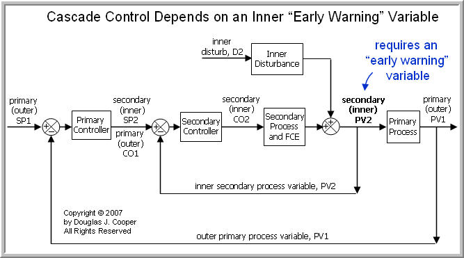
In the cascade architecture, inner secondary PV2 serves as this early warning process variable. Given this, essential design characteristics for selecting PV2 include that:
▪ it be measurable with a sensor,
▪ the same FCE (e.g., valve) used to manipulate PV1 also manipulates PV2,
▪ the same disturbances that are of concern for PV1 also disrupt PV2, and
▪ PV2 responds before PV1 to disturbances of concern and to FCE manipulations.

Since PV2 sees the disruption first, it provides our "early warning" that a disturbance has occurred and is heading toward PV1. The inner secondary controller can begin corrective action immediately. And since PV2 responds first to final control element (e.g., valve) manipulations, disturbance rejection can be well underway even before primary variable PV1 has been substantially impacted by the disturbance.

With such a cascade architecture, the control of the outer primary process variable PV1 benefits from the corrective actions applied to the upstream early warning measurement PV2.

Disturbance Must Impact Early Warning Variable PV2
As shown below (click for a large view), even with a cascade structure, there will likely be disturbances that impact PV1 but do not impact early warning variable PV2.

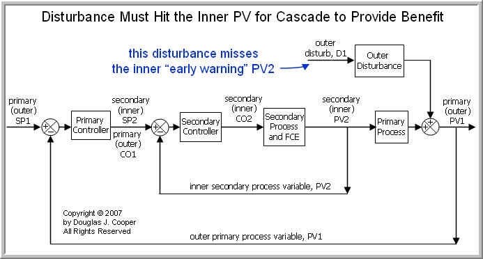
The inner secondary controller offers no "early action" benefit for these outer disturbances. They are ultimately addressed by the outer primary controller as the disturbance moves PV1 from set point.

On a positive note, a proper cascade can improve rejection performance for any of a host of disturbances that directly impact PV2 before disrupting PV1.

An Illustrative Example
To illustrate the construction and value of a cascade architecture, consider the liquid level control process shown below (click for a large view). This is a variation on our gravity drained tanks, so hopefully, the behavior of the process below follows intuitively from our previous investigations.

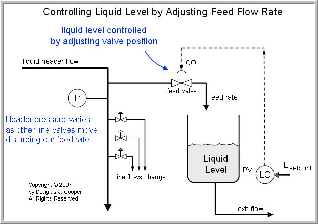
As shown above, the tank is essentially a barrel with a hole punched in the bottom. Liquid enters through a feed valve at the top of the tank. The exit flow is liquid draining freely by the force of gravity out through the hole in the tank bottom.

The control objective is to maintain liquid level at set point (SP) in spite of unmeasured disturbances. Given this objective, our measured process variable (PV) is liquid level in the tank. We measure level with a sensor and transmit the signal to a level controller (the LC inside the circle in the diagram).

After comparing set point to measurement, the level controller (LC) computes and transmits a controller output (CO) signal to the feed valve. As the feed valve opens and closes, the liquid feed rate entering the top of the tank increases and decreases to raise and lower the liquid level in the tank.

This "measure, compute and act" procedure repeats every loop sample time, T, as the controller works to maintain tank level at set point.

The Disturbance
The disturbance of concern is the pressure in the main liquid header. As shown in the diagram above, the header supplies the liquid that feeds our tank. It also supplies liquid to several other lines flowing to different process units in the plant.

Whenever the flow rate of one of these other lines changes, the header pressure can be impacted. If several line valves from the main header open at about the same time, for example, the header pressure will drop until its own control system corrects the imbalance. If one of the line valves shuts in an emergency action, the header pressure will momentarily spike.

As the plant moves through the cycles and fluctuations of daily production, the header pressure rises and falls in an unpredictable fashion. And every time the header pressure changes, the feed rate to our tank is impacted.

Problem with Single Loop Control
The single loop architecture in the diagram above attempts to achieve our control objective by adjusting valve position in the liquid feed line. If the measured level is higher than set point, the controller signals the valve to close by an appropriate percentage with the expectation that this will decrease feed flow rate accordingly.

But feed flow rate is a function of two variables:
▪ feed valve position, and
▪ the header pressure pushing the liquid through the valve (a disturbance).

To explore this, we conduct some thought experiments:

Thought Experiment #1: Assume that the main header pressure is perfectly constant over time. As the feed valve opens and closes, the feed flow rate and thus tank level increases and decreases in a predictable fashion. In this case, a single loop structure provides acceptable level control performance.

Thought Experiment #2: Assume that our feed valve is set in a fixed position and the header pressure starts rising. Just like squeezing harder on a spray bottle, the valve position can remain constant yet the rising pressure will cause the flow rate through the fixed valve opening to increase.

Thought Experiment #3: Now assume that the header pressure starts to rise at the same moment that the controller determines that the liquid level in our tank is too high. The controller can be closing the feed valve, but because header pressure is rising, the flow rate through the valve can actually be increasing.

As presented in Thought Experiment #3, The changing header pressure (a disturbance) can cause a contradictory outcome that can confound the controller and degrade control performance.

A Cascade Control Solution
For high performance disturbance rejection, it is not valve position, but rather, feed flow rate that must be adjusted to control liquid level.

Because header pressure changes, increasing feed flow rate by a precise amount can sometimes mean opening the valve a lot, opening it a little, and because of the changing header pressure, perhaps even closing the valve a bit.

Below is a classic level-to-flow cascade architecture (click for a large view). As shown, an inner secondary sensor measures the feed flow rate. An inner secondary controller receives this flow measurement and adjusts the feed flow valve.

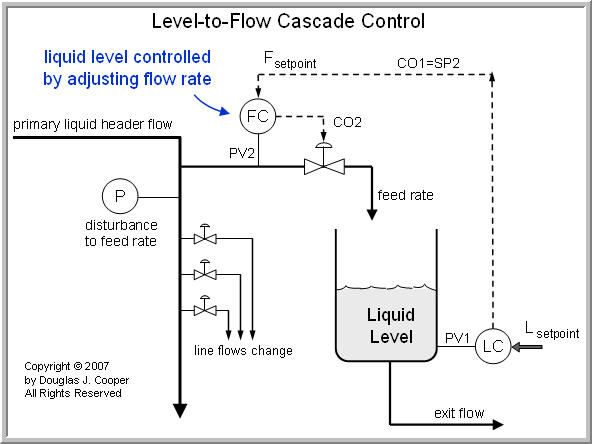
With this cascade structure, if liquid level is too high, the primary level controller now calls for a decreased liquid feed flow rate rather than simply a decrease in valve opening. The flow controller then decides whether this means opening or closing the valve and by how much.

Note in the diagram that, true to a cascade, the level controller output signal (CO1) becomes the set point for the flow controller (SP2).

Header pressure disturbances are quickly detected and addressed by the secondary flow controller. This minimizes any disruption caused by changing header pressure to the benefit of our primary level control process.

The Level-to-Flow Cascade Block Diagram
As shown in the block diagram below (click for a large view), our level-to-flow cascade fits into our block diagram structure. As required, there are:

▪ Two controllers - the outer primary level controller (LC) and inner secondary feed flow controller (FC)

▪ Two measured process variable sensors - the outer primary liquid level (PV1) and inner secondary feed flow rate (PV2)

▪ One final control element (FCE) - the valve in the liquid feed stream

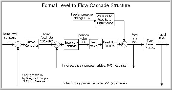
As required for a successful design, the inner secondary flow control loop is nested inside the primary outer level control loop. That is:

▪ The feed flow rate (PV2) responds before the tank level (PV1) when the header pressure disturbs the process or when the feed valve moves.

▪ The output of the primary controller, CO1, is wired such that it becomes the set point of the secondary controller, SP2.

▪ Ultimately, level measurement, PV1, is our process variable of primary concern. Protecting PV1 from header pressure disturbances is the goal of the cascade.

Design and Tuning
The inner secondary and outer primary controllers are from the PID family of algorithms. We have explored the design and tuning of these controllers in numerous articles, so as we will see, implementing a cascade builds on many familiar tasks.

There are a number of issues to consider when selecting and tuning the controllers for a cascade. We explore next an implementation recipe for cascade control.

Return to the Table of Contents to learn more.