In modern plants, process variable (PV) measurement signals are typically scaled to engineering units before they are displayed on the control room HMI computer screen or archived for storage by a process data historian. This is done for good reasons.
When operations staff walk through the plant, the assorted field gauges display the local measurements in engineering units to show that a vessel is operating, for example, at a pressure of 25 psig (1.7 barg) and a temperature of 140 oC (284 oF).
It makes sense, then, that the computer screens in the control room display the set point (SP) and PV values in these same familiar engineering units because:
| • | It helps the operations staff translate their knowledge and intuition from their field experience over to the abstract world of crowded HMI computer displays. |
| • | Familiar units will facilitate the instinctive reactions and rapid decision making that prevents an unusual occurrence from escalating into a crisis situation. |
| • | The process was originally designed in engineering units, so this is how the plant documentation will list the operating specifications. |
Controlguru.com Articles Compute Kc With Units
Like a control room display, the Controlguru.com e-book presents PV values in engineering units. In most articles, these PVs are used directly in tuning correlations to compute controller gains, Kc. As a result, the Kc values also carry engineering units.
The benefit of this approach is that controller gain maintains the intuitive familiarity that engineering units provide. The difficulty is that commercial controllers are normally configured to use a dimensionless Kc (or dimensionless proportional band, PB).
To address this issue, we explore below how to convert a Kc with engineering units into the standard dimensionless (%/%) form.
The conversion formula presented at the end of this article is reasonably straightforward to use. But it is derived from several subtle concepts that might benefit from explanation. Thus, we begin with a background discussion on units and scaling, and work our way toward our Kc conversion formula goal.
From Analog Sensor to Digital Signal
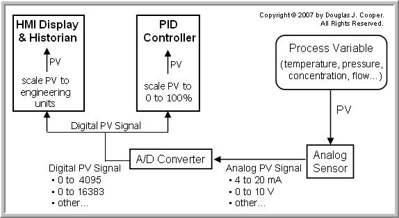
There are many ways to measure a process variable and move the signal into the digital world for use in a computer based control system. Below is a simplified sketch of one approach (click for a large view).

Other operations in the pathway from sensor to control system not shown in the simplified sketch might include a transducer, an amplifier, a transmitter, a scaling element, a linearizing element, a signal filter, a multiplexer, and more.
The central issue for this discussion is that the PV signal arrives at the computers and controllers in a raw digital form. The continuous analog PV measurement has beenquantized (broken into) a range of discrete increments or digital integer “counts” by an A/D (analog to digital) converter.
More counts dividing the span of a measurement signal increases the resolution of the measurement when expressed as a digital value. The ranges offered by most vendors result from the computer binary 2n form where n is the number of bits of resolution used by the A/D converter.
| Example: a 12 bit A/D converter digitizes an analog signal into 212 = 4096 discrete increments normally expressed to range from 0 to 4095 counts. |
| A 13 bit A/D converter digitizes an analog signal into 213 = 8192 discrete increments normally expressed to range from 0 to 8191 counts. |
| A 14 bit A/D converter digitizes an analog signal into 214 = 16384 discrete increments normally expressed to range from 0 to 16383 counts. |
| Example: if a 4 to 20 mA (milliamp) analog signal range is digitized by a 12 bit A/D converter into 0 to 4095 counts, then the resolution is: (20 – 4 mA) ÷ 4095 counts = 0.00391 mA/count |
| A signal of 7 mA from an analog range of 4 to 20 mA changes to digital counts from the 12 bit A/D converter as: (7 – 4 mA) ÷ 0.00391 mA/count = 767 counts |
| A signal of 1250 counts from a 12 bit A/D converter corresponds to an input signal of 8.89 mA from an analog range of 4 to 20 mA as: 4 mA + (1250 counts)∙(0.00391 mA/count) = 8.89 mA |
Scaling the Digital PV Signal to Engineering Units for Display
During the configuration phase of a control project, the minimum and maximum (or zero and span) of the PV measurement must be entered. These values are used to scale the digital PV signal to engineering units for display and storage.
| Example: if a temperature range of 100 oC to 500 oC is digitized into 0 to 8191 counts by a 13 bit A/D converter, the signal is scaled for display and storage by setting the minimum digital value of 0 counts = 100 oC, and maximum digital value of 8191 counts = 500 oC |
| Each digital count from the 13 bit A/D converter gives a resolution of: (500 – 100 oC) ÷ 8191 counts = 0.0488 oC/count |
| A signal of 175 oC from an analog range of 100 oC to 500 oC changes to digital counts from the 13 bit A/D converter as: (175 – 100 oC) ÷ 0.0488 oC/count = 1537 counts |
| A signal of 1250 counts from the 13 bit A/D converter corresponds to an input signal of 161 oC from an analog range of 100 oC to 500 oC as: 100 oC + (1250 counts)∙(0.0488 oC/count) = 161 oC |
As discussed at the top of this article, the intuition and field knowledge of the operations staff is maintained by using engineering units in control room displays and when storing data to a historian.
For this same reason, modern control software uses engineering units when passing variables between the function blocks used for calculations and decision-making. Calculation and decision functions are easier to understand, document and debug when the logic is written using floating point values in common engineering units.
Scaling the Digital PV Signal for Use by the PID Controller
Most commercial PID controllers use a controller gain, Kc (or proportional band, PB) that is expressed as a standard dimensionless %/%.
| Note: Controller gain in commercial controllers is often said to be unitless or dimensionless, but Kc actually has units of (% of CO signal)/(% of PV signal). In a precise mathematical world, these units do not cancel, though there is little harm in speaking as though they do. |
Prior to executing the PID controller calculation, the PV signal must be scaled to a standard 0% to 100% to match the “dimensionless” Kc. This happens every loop sample time, T, regardless of whether we are measuring temperature, pressure, flow, or any other process variable.
To perform this scaling, the minimum and maximum PV values in engineering units corresponding to the 0% to 100% standard PV range must be entered during setup and loop configuration.
| Example: if a temperature range of 100 oC to 500 oC is digitized into 0 to 8191 counts by a 13 bit A/D converter, the signal is scaled for the PID control calculation by setting the minimum digital value of 0 counts = 0%, and the maximum digital value of 8191 counts = 100%. |
| Each digital count from the 13 bit A/D converter gives a resolution of: (100 – 0%) ÷ 8191 counts = 0.0122%/count |
| A signal of 1537 counts (175 oC) from a 13 bit A/D converter would translate to a signal of 18.75% as: 0% + (1537)∙(0.0122%/value) = 18.75% |
| A signal of 1250 counts (161 oC) from a 13 bit A/D converter would translate to a signal of 15.25% as: 0% + (1250)∙(0.0122%/value) = 15.25% |
Control Output is 0% to 100%
The controller output (CO) from commercial controllers normally default to a 0% to 100% digital signal as well. Digital to analog (D/A) converters begin the transition of moving the digital CO values into the appropriate electrical current and voltage required by the valve, pump or other final control element (FCE) in the loop.
| Note: While CO commonly defaults to a 0% to 100% signal, this may not be appropriate when implementing the outer primary controller in a cascade. The outer primary CO1 becomes the set point of the inner secondary controller, and signal scaling must match. For example, if SP2 is in engineering units, the CO1 signal must be scaled accordingly. |
Care Required When Using Engineering Units For Controller Tuning
It is quite common to analyze and design controllers using data retrieved from our process historian or captured from our computer display. Just as with the articles in this e-book, this means the computed Kc values will likely be scaled in engineering units.
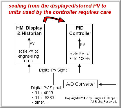
The sketch below highlights (click for a large view) that scaling from engineering units to a standard 0% to 100% range used in commercial controllers requires careful attention to detail.
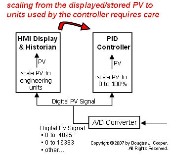
The conversion of PV in engineering units to a standard 0% to 100% range requires knowledge of the maximum and minimum PV values in engineering units. These are the same values that are entered into our PID controller software function block during setup and loop configuration. The general conversion formula is:
where:
PVmax = maximum PV value in engineering units
PVmin = minimum PV value in engineering units
PV = current PV value in engineering units
| Example: a temperature signal ranges from 100 oC to 500 oC and we seek to scale it to a range of 0% to 100% for use in a PID controller. We set: PVmin = 100 oC and PVmax = 500 oC |
| A temperature of 175 oC converts to a standard 0% to 100% range as: [(175 – 100 oC) ÷ (500 – 100 oC)]∙(100 – 0%) = 18.75% |
| A temperature of 161 oC converts to a standard 0% to 100% range as: [(161 – 100 oC) ÷ (500 – 100 oC)]∙(100 – 0%) = 15.25% |
Applying Conversion to Controller Gain, Kc
The discussion to this point provides the basis for the formula used to convert Kc from engineering units into dimensionless (%/%):
| Example: the moderate Kc value in our P-Only control of the heat exchangerstudy is Kc = – 0.7 %/ oC. For this process, PVmax = 250 oC and PVmin = 0 oC |
| Kc = (– 0.7 %/ oC)∙[(250 – 0 oC) ÷ (100 – 0%)] = – 1.75 %/% |
| Example: the moderate value for Kc in our P-Only control of the gravity drained tanks study is Kc = 8 %/ oC For this process, PVmax = 10 m and PVmin = 0 m |
| Kc = (8 %/ m)∙[(10 – 0 m) ÷ (100 – 0%)] = 0.8 %/% |
Final Thoughts
Textbooks are full of rule-of-thumb guidelines for estimating initial Kc values for a controller depending on whether, for example, it is a flow loop, a temperature loop or a liquid level loop. While we have great reservations with such a “guess and test” approach to tuning, it is important to recognize that such rules are based on a Kc that is expressed in a dimensionless (%/%) form.