By Doug Cooper and Allen Houtz1
The most popular architectures for improved disturbance rejection performance arecascade control and the “feed forward with feedback trim” architecture introduced below.
Like cascade, feed forward requires that additional instrumentation be purchased, installed and maintained. Both architectures also require additional engineering time for strategy design, implementation and tuning.
Cascade control will have a small impact on set point tracking performance when compared to a traditional single-loop feedback design and this may or may not be considered beneficial depending on the process application. The feed forward element of a “feed forward with feedback trim” architecture does not impact set point tracking performance in any way.
Feed Forward Involves a Measurement, Prediction and Action
Consider that a process change can occur in another part of our plant and an identifiable series of events then leads that “distant” change to disturb or disrupt our measured process variable, PV.
The traditional PID controller takes action only when the PV has been moved from set point, SP, to produce a controller error, e(t) = SP – PV. Thus, disruption to stable operation is already in progress before a feedback controller first begins to respond. From this view, a feedback strategy simply starts too late and at best can only work to minimize the upset as events unfold.
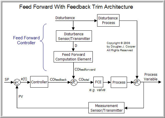
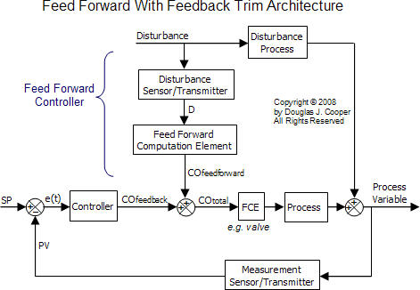
In contrast, a feed forward controller measures the disturbance, D, while it is still distant. As shown below (click for a larger view), a feed forward element receives the measured D, uses it to predict an impact on PV, and then computes preemptive control actions, COfeedforward, that counteract the predicted impact as the disturbance arrives. The goal is to maintain the process variable at set point (PV = SP) throughout the disturbance event.
where:
CO = controller output signal
D = measured disturbance variable
e(t) = controller error, SP – PV
FCE = final control element (e.g., valve, variable speed pump or compressor)
PV = measured process variable
SP = set point
To appreciate the additional components associated with a feed forward controller, we can compare the above to the previously discussed traditional feed back control loop block diagram.
When to Consider Cascade Control
The cascade architecture requires that an “early warning” secondary measured process variable, PV2, be identified that is inside (responds before) the primary measured process variable, PV1. Essential elements for success include that:
▪ PV2 is measurable with a sensor.
▪ The same final control element (FCE) used to manipulate PV1 also manipulates PV2.
▪ The same disturbances that are of concern for PV1 also disrupt PV2.
▪ PV2 responds before PV1 to disturbances of concern and to FCE manipulations.
One benefit of a cascade architecture is that it uses two traditional controllers from the PID family, so implementation is a familiar task that builds upon our existing skills. Also, cascade control will help improve the rejection of any disturbance that first disrupts the early warning variable, PV2, prior to impacting the primary process variable, PV1.
When to Consider Feed Forward with Feedback Trim
Feed forward anticipates the impact of a measured disturbance on the PV and deploys control actions to counteract the impending disruption in a timely fashion. This can significantly improve disturbance rejection performance, but only for the particular disturbance variable being measured.
Feed forward with feedback trim offers a solution for improved disturbance rejection if no practical secondary process variable, PV2, can be established (i.e., a process variable cannot be located that is measureable, provides an early warning of impending disruption, and responds first to FCE manipulations).
Feed forward also has value if our concern is focused on one specific disturbance that is responsible for repeated, costly disruptions to stable operation. To provide benefit, the additional measurement must reveal process disturbances before they arrive at our PV so we have time to compute and deploy preemptive control actions.
The Feed-Forward-Only Controller
Pure feed-forward-only controllers are rarely found in industrial applications where the process flow streams are composed of gases, liquids, powders, slurries or melts. Nevertheless, we explore this idea using a thought experiment on the shell-and-tube heat exchanger simulation detailed in a previous article and available for exploration and study in commercial software.
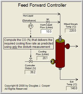
The architecture of a feed-forward-only controller for the heat exchanger is illustrated below (click for a larger view):

As detailed in the referenced article, the PV to be controlled is the exit temperature on the tube side of the exchanger. To regulate this exit temperature, the CO signal adjusts a valve to manipulate the flow rate of cooling liquid on the shell side. A side stream of warm liquid combines with the hot liquid entering the exchanger and acts as a measured disturbance, D, to our process.
Because there is no feedback of a PV measurement in our controller architecture, feed-forward-only presents the interesting notion of open loop control. As such, it does not have a tendency to induce oscillations in the PV as can a poorly tuned feedback controller.
If we could mathematically describe how each change in D impacts PV (D −› PV) and how each change in CO impacts PV (CO −› PV), then we could develop a math model that predicts what manipulations to make in CO to maintain PV at set point whenever D changes.
But this would only be true if:
▪ we have perfect understanding of the D −› PV and CO −› PV dynamic relationships,
▪ we can describe these perfect dynamic relationships mathematically,
▪ these relationships never change,
▪ there are no other unmeasured disturbances impacting PV, and
▪ set point, SP, is always held constant.
The reality, however, is that with only a single measured D, a predictive model cannot account for many phenomena that impact the D −› PV and CO −› PV behavior. These may include changes in:
| ▪ | the temperature and flow rate of the hot liquid feed that mixes with our warm disturbance stream on the tube side, |
| ▪ | the temperature of the cooling liquid on the shell side, |
| ▪ | the ambient temperature surrounding the exchanger that drives heat loss to the environment, |
| ▪ | the shell/tube heat transfer coefficient due to corrosion or fouling, and |
| ▪ | valve performance and capability due to wear and component failure. |
Since all of the above are unmeasured, a fixed or stationary model cannot account for them when it computes control action predictions. Installing additional sensors and enhancing the feed forward model to account for each would improve performance but would lead to an expensive and complex architecture.And since there are more potential disturbances and external influences then those listed above, that still would not be sufficient.
This highlights that feed-forward-only control is problematic and should only be considered in rare instances. One situation where it may offer value is if a PV critical to process operation simply cannot be measured or inferred using currently available technology. Feed-forward-only control, in spite of its weaknesses and pitfalls, then offers some potential for improved operation.
Feed Forward with Feedback Trim
The “feed forward with feedback trim” control architecture is the solution widely employed in industrial practice. It balances the capability of a feed forward element to take preemptive control actions for one particularly disruptive disturbance while permitting a traditional feedback control loop to:
| ▪ | reject all other disturbances and external influences that are not measured, |
| ▪ | provide set point tracking capability, and |
| ▪ | correct for the inevitable simplifying approximations in the predictive model of the feed forward element that make preemptive disturbance rejection imperfect. |
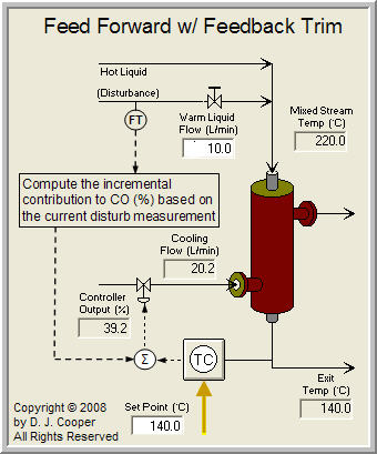
A feed forward with feedback trim control architecture for the heat exchanger process is shown below (click for a larger view):

To construct the architecture, a feedback controller is first implemented and tested following our controller design and tuning recipe as if it were a stand-alone entity. The feed forward controller is then designed based on our understanding of the relationshipbetween the D −› PV and CO −› PV variables. This is generally expressed as a math function that can range in complexity from a simple multiplier to complex differential equations.
With the architecture completed, the disturbance flow is measured and passed to a feed forward element that is essentially a combination disturbance/process model. The model uses changes in D to predict an impact on PV, and then computes control actions, COfeedforward to compensate for the predicted impact.
Conceptual Feed Forward with Feedback Trim Diagram
As shown in the first block diagram above, the COfeedforward control actions are combined with COfeedback to create an overall control action, COtotal, to send to the final control element (FCE).
To illustrate the control strategy in a more tangible fashion, we present the feed forward with feedback trim architecture in a conceptual diagram below (click for a larger view):
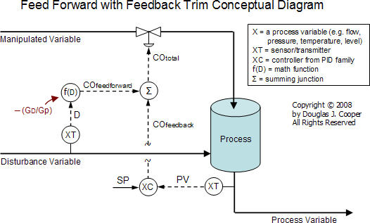
The basis for the feed forward element math function, f(D) = ─ (GD/Gp) shown in the diagram is discussed in detail in this next article.
The more accurate the feed forward math function is in computing control actions that will counteract changes in the measured disturbance in a timely fashion, the less impact those disturbances will have on our measured process variable.
| Practitioner’s note: a potential application of feed forward control exists if we hear an operator say something like, “Every time event A happens, process variable X is upset. I can usually help the X controller by switching to manual mode and moving the controller output.” If the variable associated with event A is already being measured and logged in the process control system, sufficient data is likely available to allow the implementation of a feed forward element to our feedback controller. |
Improved disturbance rejection performance comes at a price in terms of process engineering time for model development and testing, and instrument engineering time for control logic programming. Like all projects, such investment decisions are made on the basis of cost and benefit.
____
1. Allen D. Houtz
Consulting Engineer
Automation Systems Group
P.O. Box 884
Kenai, AK 99611
Email: ifadh@uaa.alaska.edu