Step 3 of our controller design and tuning recipe is to approximate the often complex behavior contained in our dynamic process test data with a simple first order plus dead time (FOPDT) dynamic model.
In this article we focus on process dead time, Өp, and seek to understand what it is, how it is computed, and what it implies for controller design and tuning. Corresponding articles present details of the other two FOPDT model parameters: process gain, Kp; and process time constant, Tp.
Dead Time is the Killer of Control
Dead time is the delay from when a controller output (CO) signal is issued until when the measured process variable (PV) first begins to respond. The presence of dead time,Өp, is never a good thing in a control loop.
Think about driving your car with a dead time between the steering wheel and the tires. Every time you turn the steering wheel, the tires do not respond for, say, two seconds. Yikes.
For any process, as Өp becomes larger, the control challenge becomes greater and tight performance becomes more difficult to achieve. “Large” is a relative term and this is discussed later in this article.
Causes for Dead Time
Dead time can arise in a control loop for a number of reasons:
| ▪ | Control loops typically have “sample and hold” measurement instrumentation that introduces a minimum dead time of one sample time, T, into every loop. This is rarely an issue for tuning, but indicates that every loop has at least some dead time. |
| ▪ | The time it takes for material to travel from one point to another can add dead time to a loop. If a property (e.g. a concentration or temperature) is changed at one end of a pipe and the sensor is located at the other end, the change will not be detected until the material has moved down the length of the pipe. The travel time is dead time. This is not a problem that occurs only in big plants with long pipes. A bench top process can have fluid creeping along a tube. The distance may only be an arm’s length, but a low enough flow velocity can translate into a meaningful delay. |
| ▪ | Sensors and analyzer can take precious time to yield their measurement results. For example, suppose a thermocouple is heavily shielded so it can survive in a harsh environment. The mass of the shield can add troublesome delay to the detection of temperature changes in the fluid being measured. |
| ▪ | Higher order processes have an inflection point that can be reasonably approximated as dead time for the purpose of controller design and tuning. Note that modeling for tuning with the simple FOPDT form is different from modeling for simulation, where process complexities should be addressed with more sophisticated model forms (all subjects for future articles). |
Sometimes dead time issues can be addressed through a simple design change. It might be possible to locate a sensor closer to the action, or perhaps switch to a faster responding device. Other times, the dead time is a permanent feature of the control loop and can only be addressed through detuning or implementation of a dead time compensator (e.g. Smith predictor).
Heat Exchanger Test Data
We seek to understand Kp by analyzing step test data from a heat exchanger. The heat exchanger is a realistic simulation where the measured process variable (PV) is the temperature of hot liquid exiting the exchanger. To regulate this PV, the controller output (CO) moves a valve to manipulate the flow rate of a cooling liquid into the exchanger.
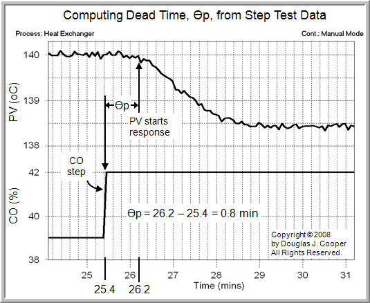
The step test data below (click for a larger view) was generated by moving the process from one steady state to another. In particular, CO was stepped from 39% up to 42%, causing the measured PV to decrease from 140 °C down to approximately 138.4 °C.
Computing Dead Time
Estimating dead time, Өp, from step test data is a three step procedure:
1. Locate the point in time when the “PV starts a clear response” to the step change in the CO. This is the same point we identified when we computed Tp in the previous article.
2. Locate the point in time when the CO was stepped from its original value to its new value.
3. Dead time, Өp, is the difference in time of step 1 minus step 2.
Applying the three step procedure to the step test plot above:
1. As we had determined in the previous Tp article, the PV starts a clear response to the CO step at 26.2 min.
2. Reading off the plot, the CO step occurred at 25.4 min, and thus,
3. Өp = 26.2 – 25.4 = 0.8 min
We analyze step test data here to make the computation straightforward, but please recognize that dead time describes “how much delay” occurs from when any sort of CO change is made until when the PV first responds to that change.
Like a time constant, dead time has units of time and must always be positive. For the types of processes explored on this site (streams comprised of gasses, liquids, powders, slurries and melts), dead time is most often expressed in minutes or seconds.
During a dynamic analysis study, it is best practice to express Tp and Өp in the same units (e.g. both in minutes or both in seconds). The tuning correlations and design rules assume consistent units. Control is challenging enough without adding computational error to our problems.
Implications for Control
• Dead time, Өp, is large or small only in comparison to Tp, the clock of the process. Tight control becomes more challenging when Өp > Tp. As dead time becomes much greater than Tp, a dead time compensator such as a Smith predictor offers benefit. A Smith predictor employs a dynamic process model (such as an FOPDT model) directly within the architecture of the controller. It requires additional engineering time to design, implement and maintain, so be sure the loop is important to safety or profitability before undertaking such a project.
• It is more conservative to overestimate dead time when the goal is tuning. ComputingӨp requires a judgment of when the “PV starts a clear response.” If your judgment says that the “clear response” is sooner in time (maybe you choose 26.0 min for this case), then Tp increases, but dead time, Өp, decreases by the same amount (and vice versa). We can see the impact this has by looking ahead to the PI tuning correlations:
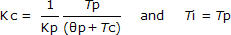
Where:
Kc = controller gain, a tuning parameter
Ti = reset time, a tuning parameter
Since Өp is in the denominator of the Kc correlation, as dead time gets larger, the controller gain gets smaller. A smaller Kc implies a less active controller. Overly aggressive controllers cause more trouble than sluggish controllers, at least in the first moments after being put into automatic. Hence, a larger dead time estimate is a more cautious or conservative estimate.
| Practitioner’s Note on the “Өp,min = T” Rule for Controller Tuning:Consider that all controllers measure, act, then wait until next sample time; measure, act, then wait until next sample time. This “measure, act, wait” procedure has a delay (or dead time) of one sample time, T, built naturally into its structure.
Thus, the minimum dead time, Өp, in any real control implementation is the loop sample time, T. Dead time can certainly be larger than T (and it usually is), but it cannot be smaller.Thus, if our model fit yields Өp < T (a dead time that is less than the controller sample time), we must recognize that this is an impossible outcome. Best practice in such a situation is to substitute Өp = T everywhere when using our controller tuning correlations and other design rules. This is the “Өp,min = T” rule for controller tuning. Read more details about the impact of sample time on controller design and tuning in this article. |