The question arises quite often, “What is the normal or standard form of the PID (proportional-integral-derivative) algorithm?”
The answer is both simple and complex. Before we explore the answer, consider the screen displays shown below (click for a large view of example 1 or example 2):
 |
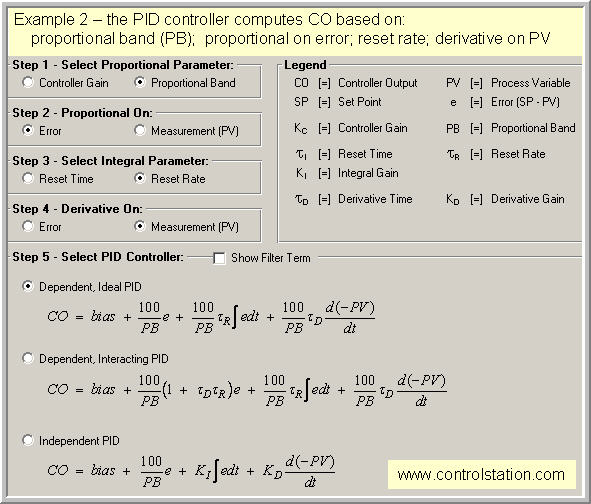 |
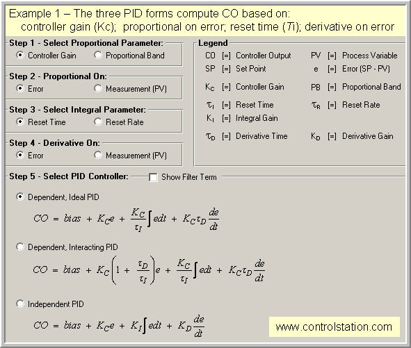
As shown in the screen displays:
▪ There are three popular PID algorithm forms (see step 5 in the large image views).
▪ Each of the three algorithms has tuning parameters and algorithm variables that can be cast in different ways (see steps 1 – 4 in the large image views).
So your vendor might be using one of dozens of possible algorithm forms. And if you add a filter term to your controller, the number of possibilities increases substantially.
The Simple Answer
Any of the algorithms can deliver the same performance as any of the others. There is no control benefit from choosing one form over another. They are all standard or normal in that sense.
If you are considering a purchase, select the vendor that serves your needs the best and don’t dwell on the specifics of the algorithm. Some things to consider include:
▪ compatibility with existing controllers and associated hardware and software
▪ cost
▪ ease of installation and maintenance
▪ reliability
▪ your operating environment (is it clean? cool? dry?)
A More Complete Answer
Most of the different controller algorithm forms can be found in one vendor’s product or another. Some vendors even use different forms within their own product lines. More information can be found in this article.
And while the various forms are equally capable, each must be tuned (values for the adjustable parameters must be specified) using tuning correlations specifically designed for that particular control algorithm.
Commercial software makes it straightforward to get desired performance from any of them. But it is essential that you know your vendor and controller model number to ensure a correct match between controller form and computed tuning values.
The alternative to an orderly design methodology is a “guess and test” approach. While used by some practitioners, such trial and error tuning squanders valuable production time, consumes more feedstock and utilities than is necessary, generates additional waste and off-spec product, and can even present safety concerns.
In most articles on Controlguru.com, we use some variation of the dependent, ideal PID controller form:
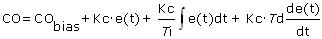
Where:
CO = controller output signal
CObias = controller bias
e(t) = current controller error, defined as SP – PV
SP = set point
PV = measured process variable
Kc = controller gain, a tuning parameter
Ti = reset time, a tuning parameter
Td = derivative time, a tuning parameter
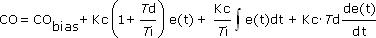
To reinforce that the controllers all are equally capable, we occasionally use variations of the dependent, interacting form:
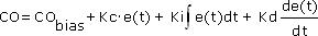
or variations of the independent PID form:
Final Thoughts
The discussion above glosses over some of the subtle differences in algorithm form that we can exploit to improve control performance. We will learn about these details as we progress in our learning.
For example, derivative on error behaves different from derivative on measured PV. This is true for all of the algorithms. Derivative on error can “kick” after set point steps and this is rarely considered desirable behavior. Thus, derivative on PV is recommended for industrial applications.
And if you are considering programming the controller yourself, it is not the algorithm form that is the challenge. The big hurdle is properly accounting for the anti-reset windup and jacketing logic to allow bumpless transition between operating modes.