Step 3 of our controller design and tuning recipe is to approximate the often complex behavior contained in our dynamic process test data with a simple first order plus dead time (FOPDT) dynamic model.
In this article we focus on process gain, Kp, and seek to understand what it is, how it is computed, and what it implies for controller design and tuning. Corresponding articles present details of the other two FOPDT model parameters: process time constant, Tp; and process dead time, Өp.
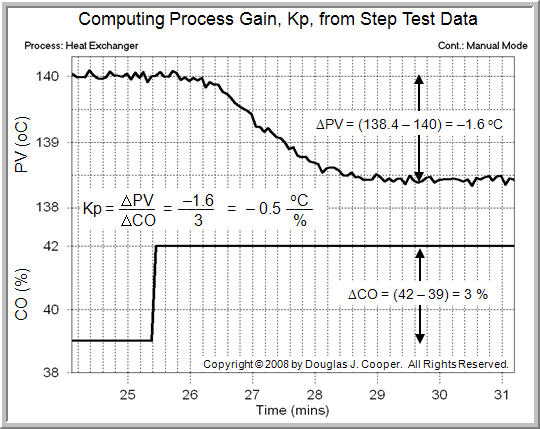
Heat Exchanger Step Test Data
We explore Kp by analyzing step test data from a heat exchanger. The heat exchanger is a realistic simulation where the measured process variable (PV) is the temperature of hot liquid exiting the exchanger. To regulate this PV, the controller output (CO) signal moves a valve to manipulate the flow rate of a cooling liquid into the exchanger.
The step test data below (click for large view) was generated by moving the process from one steady state to another. As shown, the CO was stepped from 39% up to 42%, causing the measured PV to decrease from 140 °C down to approximately 138.4 °C.
Computing Process Gain
Kp describes the direction PV moves and how far it travels in response to a change in CO. It is based on the difference in steady state values. The path or length of time the PV takes to get to its new steady state does not enter into the Kp calculation.
Thus, Kp is computed:

where ΔPV and ΔCO represent the total change from initial to final steady state.
| Aside: the assumptions implicit in the discussion above include that: ▪ the process is properly instrumented as a CO to PV pair, ▪ major disturbances remained reasonably quiet during the test, and ▪ the process itself is self regulating. That is, it naturally seeks to run at a steady state if left uncontrolled and disturbances remain quiet. Most, but certainly not all, processes are self regulating. Certain configurations of something as simple as liquid level in a pumped tank can be non-self regulating. |
Reading numbers off the above plot:
| ▪ | The CO was stepped from 39% up to 42%, so the ΔCO = 3%. |
| ▪ | The PV was initially steady at 140 °C and moved down to a new steady state value of 138.4 °C. Since it decreased, the ΔPV = –1.6 °C. |
Using these ΔCO and ΔPV values in the Kp equation above, the process gain for the heat exchanger is computed:
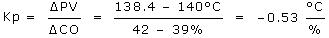
| Practitioner’s Note: Real plant data is rarely as clean as that shown in the plot above and we should be cautious not to try and extract more information from our data than it actually contains. When used in tuning correlations, rounding the Kp value to –0.5 °C/% will provide virtually the same performance. |
Kp Impacts Control
Process gain, Kp, is the “how far” variable because it describes how far the PV will travel for a given change in CO. It is sometimes called the sensitivity of the process.
If a process has a large Kp, then a small change in the CO will cause the PV to move a large amount. If a process has a small Kp, the same CO change will move the PV a small amount.
As a thought experiment, let’s suppose a disturbance moves our measured PV away from set point (SP). If the process has a large Kp, then the PV is very sensitive to CO changes and the controller should make small CO moves to correct the error. Conversely, if the process has a small Kp, then the controller needs to make large CO actions to correct the same error.
This is the same as saying that a process with a large process gain, Kp, should have a controller with a small controller gain, Kc (and vice versa).
Looking ahead to the PI tuning correlations we will use in our case studies:
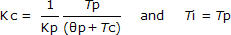
Where:
Kc = controller gain, a tuning parameter
Ti = reset time, a tuning parameter
Notice that in the Kc correlation, a large Kp in the denominator will yield a small Kc value (that is, Kc is inversely proportional to Kp). Thus, the tuning correlation tells us the same thing as our thought experiment above.
Sign of Kp Tells Direction
The sign of Kp tells us the direction the PV moves relative to the CO change. The negative value found above means that as the CO goes up, the PV goes down. We see this “up-down” relationship in the plot. For a process where a CO increase causes the PV to move up, the Kp would be positive and this would be an “up-up” process.
When implementing a controller, we need to know if our process is up-up or up-down. If we tell the controller the wrong relationship between CO actions and the direction of the PV responses, our mistake may prove costly. Rather than correcting for errors, the controller will quickly amplify them as it drives the CO signal, and thus the valve, pump or other final control element (FCE), to the maximum or minimum value.
Units of Kp
If we are computing Kp and want the results to be meaningful for control, then we must be analyzing wire out to wire in CO to PV data as used by the controller.
The heat exchanger data plot indicates that the data arriving on the PV wire into the controller has been scaled (or is being scaled in the controller) into units of temperature. And this means the the controller gain, Kc, needs to reflect the units of temperature as well.
This may be confusing, at least initially, since most commercial controllers do not require that units be entered. The good news is that, as long as our computations use the same “wire out to wire in” data as collected and displayed by our controller, the units will be consistent and we need not dwell on this issue.
| Aside: for the Kc tuning correlation above, the units of time (dead time and time constants) cancel out. Hence, the controller gain, Kc, will have the reciprocal or inverse units of Kp. For the heat exchanger, this means Kc has units of %/°C.With modern computer control systems, scaling for unit conversions is becoming more common in the controller signal path. Sometimes a display has been scaled but the signal in the loop path has not. You must pay attention to this detail and make sure you are using the correct units in your computations. There is more discussion in this article.It has been suggested that the gain of some controllers do not have units since both the CO and PV are in units of %. Actually, the Kc will have units of “% of CO signal” divided by “% of PV signal,” which mathematically do not cancel out. |
| Practitioner’s Note: Step test data is practical in the sense that all model fitting computations can be performed by reading numbers off of a plot. However, when dealing with production processes, operations personnel tend to prefer quick “bumps” rather than complete step tests.Step tests move the plant from one steady state to another. This takes a long time, may have safety implications, and can create expensive off-spec product. Pulse and doublet tests are examples of quick bumps that returns our plant to desired operating conditions as soon as the process data shows a clear response to a controller output (CO) signal change.Getting our plant back to a safe, profitable operation as quickly as possible is a popular concept at all levels of operation and management. Using pulse tests requires the use of inexpensive commercial software to analyze the bump test results, however. |