In recent articles, we investigated P-Only control and then PI control of a heat exchanger. Here we explore the benefits and challenges of derivative action with a PID control study of this process. Our focus is on basic design, implementation and performance issues.
We follow the same four-step design and tuning recipe we use for all control implementations. A benefit of the recipe, beyond the fact that it is easy to use, widely applicable, and reliable in industrial applications, is that steps 1-3 of the recipe remain the same regardless of the control algorithm being employed.
Summary results of steps 1-3 from the previous heat exchanger control studies are presented below. Details for these steps are presented with discussion in the PI control article (nomenclature for this article is listed in step 4).
Step 1: Specify the Design Level of Operation (DLO)
▪ Design PV and SP = 138 °C with operation ranging from 138 to 140 °C
▪ Expected warm liquid flow disturbance = 10 L/min
Step 2: Collect Process Data around the DLO
See the PI control article referenced above for a summary, or go to this article to see details of the data collection experiment.
Step 3: Fit an FOPDT Model to the Dynamic Data
The first order plus dead time (FOPDT) model approximation of the heat exchanger data from step 2 is:
▪ Process gain (how far), Kp = –0.53 °C/%
▪ Time constant (how fast), Tp = 1.3 min
▪ Dead time (how much delay), Өp = 0.8 min
Step 4: Use the Parameters to Complete the Design
Vendors market the PID algorithm in a number of different forms, creating a confusing array of choices for the practitioner.
The preferred algorithm in industrial practice is PID with derivative on PV. The three most common of these forms each have their own tuning correlations, and they all provide identical performance as long as we take care to match each algorithm with its proper correlations during implementation.
Because the three common forms are identical in capability and performance if properly tuned, the observations and conclusions we draw from any one of these algorithms applies to the other forms.
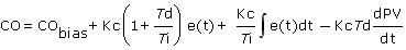
Among the most widely used is the Dependent, Ideal (Non-interacting) form:
![]()
Where:
CO = controller output signal (the wire out)
CObias = controller bias; set by bumpless transfer
e(t) = current controller error, defined as SP – PV
SP = set point
PV = measured process variable (the wire in)
Kc = controller gain, a tuning parameter
Ti = reset time, a tuning parameter
Td = derivative time, a tuning parameter
As explained in the PI control study, best practice is to set loop sample time, T, at 10 times per time constant or faster (T ≤ 0.1Tp). For this process, controller sample time, T = 1.0 sec. Also, like most commercial controllers, we employ bumpless transfer. Thus, when switching to automatic, SP is set equal to the current PV and CObias is set equal to the current CO.
• Controller Gain, Reset Time & Derivative Time
We use the industry-proven Internal Model Control (IMC) tuning correlations in this study. These require specifying the closed loop time constant, Tc, that describes the desired speed or quickness of our controller in responding to a set point change or rejecting a disturbance.
Guidance for computing Tc for an aggressive, moderate or conservative controller action are listed in our PI control study and summarized as:
▪ aggressive: Tc is the larger of 0.1·Tp or 0.8·Өp
▪ moderate: Tc is the larger of 1·Tp or 8·Өp
▪ conservative: Tc is the larger of 10·Tp or 80·Өp
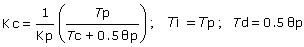
With Tc determined, the IMC tuning correlations for the Dependent, Ideal (Non-Interacting) PID form are:
Note that, similar to the PI controller tuning correlations, only controller gain containsTc, and thus, only Kc changes based on a desire for a more active or less active controller.
We start our study by choosing an aggressive response tuning:
Aggressive Tc = the larger of 0.1·Tp or 0.8·Өp
= larger of 0.1 (1.3 min) or 0.8 (0.8 min)
= 0.64 min
Using this Tc and our Kp, Tp and Өp from Step 3 in the correlations above, we compute these aggressive PID tuning values:
Aggressive Ideal PID: Kc = –3.1 %/°C; Ti = 1.7 min; Td = 0.31 min
• Controller Action
Controller gain is negative for the heat exchanger, yet most commercial controllers require that a positive value of Kc be entered. The way we indicate a negative sign is to choose the direct acting controller option during implementation. If the wrong control action is entered, the controller will quickly drive the final control element to full on/open or full off/closed and remain there until a proper control action entry is made.
| Practitioner’s Note: Controller gain, Kc, always has the same sign as the process gain, Kp. For a process with a negative Kp such as our heat exchanger, when the CO increases, the PV decreases (sometimes called up-down behavior). With the controller in automatic, if the PV is too high, the controller has to increase CO to correct for the error. The CO acts directly toward the problem, and thus, is said to be direct acting. If Kp (and thus Kc) are positive or up-up, when the PV is too high, the controller has to decrease CO to correct for the error. The CO acts in reverse of the problem and is said to be reverse acting. |
Implement and Test
Below we compare the performance of two controllers side-by-side for the heat exchanger process simulation (click for large view). Shown are two set point step pairs from 138 °C up to 140 °C and back again. Though not shown, the disturbance flow rate remains constant at 10 L/min throughout the study.To the left is set point tracking performance for an aggressively tuned PI controller from our previous study. To the right is the set point tracking performance of our aggressively tuned PID controller.
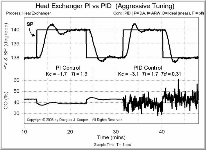
The PID controller not only displays a faster rise time (because Kc is bigger), but also a faster settling time. This is because derivative action seeks to inhibit rapid movements in the process variable. One result of this is a decrease in the rolling or oscillatory behavior in the PV trace.
Perhaps more significant, however, is the obvious difference in the CO signal trace for the two controllers. Derivative action causes the noise (random error) in the PV signal to be amplified and reflected in the control output. Such extreme control action will wear a mechanical final control element, requiring increased maintenance.
This unfortunate consequence of noise in the measured PV is a serious disadvantage with PID control. We will discuss this more in the next article.
Tune One, Tune Them All
To complete this study, we compare the Dependent, Ideal (Non-interacting) form above to the performance of the Dependent, Interacting form:
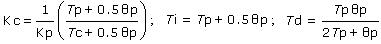
The IMC tuning correlations for this form are:
For variety, we explore moderate response tuning:
Moderate Tc = the larger of 1·Tp or 8·Өp
= larger of 1 (1.3 min) or 8 (0.8 min)
= 6.4 min
Using this Tc and our model parameters in the proper tuning correlations, we arrive at these moderate tuning values:
Dependent, Interacting PID: Kc = –0.36 %/°C; Ti = 1.3 min; Td = 0.40 min
Dependent, Ideal PID: Kc = –0.47 %/°C; Ti = 1.7 min; Td = 0.31 min
As shown in the plot below (click for a large view), we see that moderate tuning provides a reasonably fast PV response while producing no overshoot.
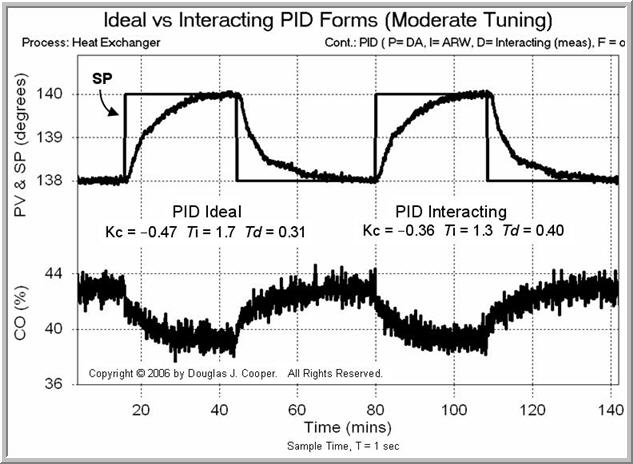
But more important, we establish that the interacting PID form and the ideal PID form provide identical performance when tuned with their own correlations.