By Bob Rice¹ and Doug Cooper

The case studies on this site largely focus on the control of self regulating processes. The principal characteristic that makes a process self regulating is that it naturally seeks a steady state operating level if the controller output and disturbance variables are held constant for a sufficient period of time.

Cruise control of a car is a self regulating process. If we keep the fuel flow to the engine constant while traveling on flat ground on a windless day, the car will settle out at some constant speed. If we increase the fuel flow rate a fixed amount, the car will accelerate and then steady out at a different constant speed.

The heat exchanger process that has been studied on this site is self regulating. If the exchanger cooling rate and disturbance flow rate are held constant at fixed values, the exit temperature will steady at a constant value. If we increase the cooling rate, wait a bit, and then return it to its original value, the exchanger exit temperature will respond during the experiment and then return to its original steady state.

But some processes where the streams are comprised of gases, liquids, powders, slurries and melts do not naturally settle out at a steady state operating level. Process control practitioners refer to these as non-self regulating, or more commonly, as integrating processes.

Integrating (non-self regulating) processes can be remarkably challenging to control. After exploring the distinctive behaviors illustrated below, you may come to realize that some of the level, temperature, pressure, pH and other loops you work with have such a character.

Integrating (Non-Self Regulating) Behavior in Manual Mode
The upper plot below shows the open loop (manual mode) behavior of the more common self regulating process. In this idealized response, the controller output (CO) and process variable (PV) are initially at steady state. The CO is stepped up and back from this steady state. As shown, the PV responds to the step, but ultimately returns to its original operating level.

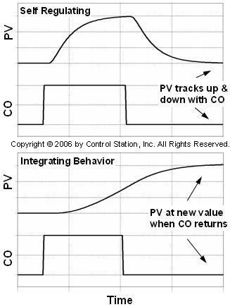
The lower plot above shows the open loop response of an ideal integrating process. The distinctive behavior is that the PV settles at a new operating level when the CO returns to its original value.

In truth, the integrating behavior plot above is misleading in that it implies that for such processes, a steady CO will produce a steady PV. While possible with idealized simulations like that used to generate the plot, such a "balance point" behavior is rarely found in open loop (manual mode) for integrating processes in an industrial operation.

More realistically, if left uncontrolled, the lack of a balance point means the PV of an integrating process will naturally tend to drift up or down, possibly to extreme and even dangerous levels. Consequently, integrating processes are rarely operated in manual mode for very long.

Aside: the behavior shown in the integrating plot can also appear across small regions of operation of a self-regulating process if there is a significant dead-band in the final control element (FCE). This might result, for example, from loose mechanical linkages in a valve. For this investigation, we assume the FCE operates properly.

P-Only Control Behavior is Different
To appreciate the difference in behavior for integrating processes, we first recall P-Only control of a self regulating process (theory discussion here and application case studies here and here). We summarize some of the lessons learned in those articles by presenting the P-Only control of an ideal self regulating simulation.

As shown below (click for a large view), when the set point (SP) is initially at the design level of operation (DLO) in the first moments of operation, then PV equals SP. Recall that the DLO is where we expect the SP and PV to be during normal operation when the major disturbances are at their normal or typical values.

The set point is then stepped up from the DLO on the left half of the plot. The simple P-Only controller is unable to track the changing SP and a steady error, called offset, results. The offset grows as each step moves the SP farther away from the DLO.

Midway through the plot, a disturbance occurs. Its size was pre-calculated in this ideal simulation to eliminate the offset. The SP is then stepped back down to the right in the plot and we see that offset shifts, but again grows in a similar and predictable pattern. 

With this as background, we next consider an ideal integrating process simulation under P-Only control as shown below (click for a large view).

Even under simple P-Only control as shown in the left half of the plot, the PV is able to track the SP steps with no offset. This behavior can be quite confusing as it does not fit the expected behavior we have just seen above for the more common self regulating process.

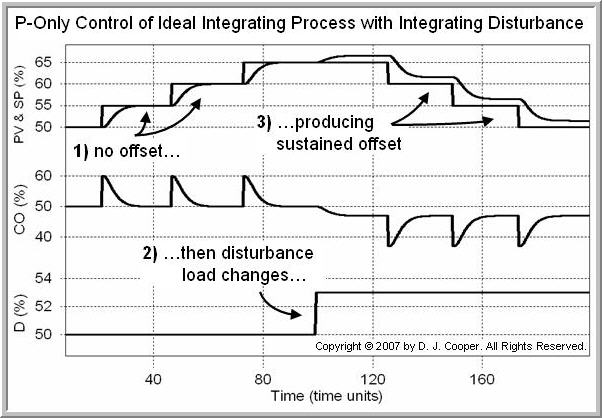
The reason this happens is that integrating processes have a natural accumulating character. In fact, this is why “integrating process” is used as a descriptor for non-self regulating processes. Since the process integrates, then it appears that the controller does not need to.

Yet the set point steps to the right in the above plot show that this is not completely correct. Once a disturbance shifts the baseline operation of the process, shown roughly at the midpoint in the above plot, an offset develops and remains constant, even as SP returns to its original design value.

Controller Output Behavior is Telling
If we study the CO trace in the two plots above, we see one feature that distinguishes self regulating from integrating process behavior.

In the self regulating process plot above, the average CO value tracks up and then down as the SP steps up and then down.

In the integrating process plot above, the CO spikes with each SP step, but then in a most unintuitive fashion, returns to the same steady value. It is only the change in the disturbance flow that causes the average CO to shift midway through the plot, though it then remains centered around the new value for the remainder of the SP steps.

PI Control Behavior is Different
The plot below (click for a large view) shows the ideal self regulating process controlled using the popular dependent ideal PI algorithm. Reset time, Ti, is held constant throughout the experiment while controller gain, Kc, is doubled and then doubled again.

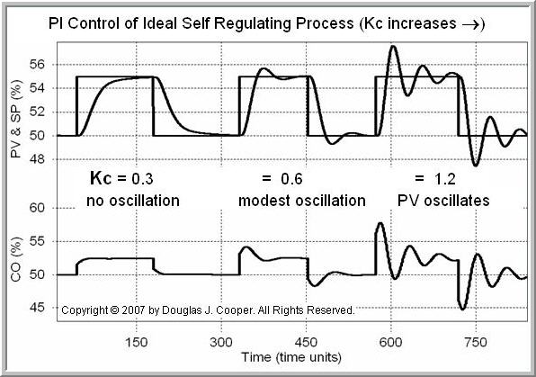
As Kc increases, the controller becomes more active, and as we have grown to expect, this increases the tendency of the PV to display oscillating (or underdamped) behavior.

For comparison, now consider PI control of an ideal integrating process simulation as shown below (click for a large view). As above, reset time, Ti, is held constant throughout the experiment while controller gain, Kc, is increased across the plot.

A counter-intuitive result is that as Kc becomes small and as it becomes large, the PV begins displaying an underdamped (oscillating) response behavior.

While the frequency of the oscillations is clearly different between a small and large Kc when seen together in a single plot as above, it is not always obvious what direction controller gain needs to move to settle the process when looking at such unacceptable performance on a control room display.

Tuning Recipe Required
One of the biggest challenges for practitioners is recognizing that a particular process shows integrating behavior prior to starting a controller design and tuning project. This, like most things, comes with training, experience and practice.

Once in automatic, closed loop behavior of an integrating process can be unintuitive and even confounding. Trial and error tuning can lead us in circles as we try to understand what is causing the problem.

A formal controller design and tuning recipe for integrating processes helps us overcome these issues in an orderly and reliable fashion.

Return to the Table of Contents to learn more.

_______
1.  Bob Rice holds primary responsibility at Control Station for training and software development, deployment, and support. Dr. Rice has published extensively on topics associated with automatic process control, including non-self-regulating processes and model predictive control. Prior to joining Control Station, Dr. Rice held engineering and technical positions with PPG Industries and The Walt Disney Company.

Robert Rice, Ph.D.
Director of Solutions Engineering
Control Station, Inc.
One Technology Drive
Tolland, CT 06084

Phone: (860) 872-2920
Email: bob.rice@controlstation.com
Web: http://www.controlstation.com/

Copyright © 2007 by Douglas J. Cooper. All Rights Reserved.