By Peter Nachtwey1
Since most of us don’t have our own heat exchanger to test on, I thought it would be good to show how one can be simulated. This would allow us to test the equations that calculate the PI tuning values over the range from a conservative to aggressive response. In addition, the sample period can be changed to see the affect that the sample period has on the response.
Building the Discrete Time Model
Learning how to model a first order plus dead time (FOPDT) system is the easiest place to start. This model simply uses the last process variable (PV) and the new CO (control output) to estimate what the new value of PV will be in the next time period.
The form of the discrete time model is:
PV(n+1) = A·PV(n) + B·Kp·CO(n–Өp) + C
The FOPDT model is basically a simple single pole filter similar to an RC circuit in electronics, except here:
1. the system has gain, Kp
2. the input at time n affects the output at time n+1
3. the system has an initial steady state, C, that is not 0
4. the system has dead time, Өp
The first thing that must be done is to build the basic model by specifying the A and B constants. Note that A and B are constants for a first order system and are arrays for higher order systems. So in this study:
A = exp(–T/Tp)
B = (1 – A)
T is the sample period and Tp is the plant time constant. A and B are coefficients in the range from 0 to 1, and coefficient A tends to be close to 1.
Calculating coefficient C in the above model is the tricky part. The heat exchanger steady state is not 0 °C. If coefficient C is left out the above model equation or it is set to zero, than PV will approach 0. This does not match the observed behavior of the heat exchanger. Therefore, a value for C must be calculated that will provide the correct value of PV when CO is set to 0.
This is done as follows. From the heat exchanger data plot, we can see that the heat exchanger temperature (PV) is 140 °C degrees when the controller output (CO) is 39%. If these values are plugged into the formula y=mx+b, we can solve for the steady state temperature, PVss:
140 = 39Kp + PVss
And this lets us calculate coefficient C:
C = (1 – A) PVss
The data below is from the Validating Our Heat Exchanger FOPDT Model tutorial. The heat exchanger is modeled as a reverse acting FOPDT system with Laplace domain transfer function:
![]()
The model parameter values for Kp, Tp and Өp where provided in the tutorial as:
• Plant gain, Kp = –0.533 °C/%
• Time constant, Tp = 1.3 min
• Dead time, Өp = 0.8 min
Also,
• Sample time, T = 1/60 min
• Dead time in samples = nӨp = Өp/T = 48
Steady state PV can now be computed assuming the system is linear:
PVss = 140 – 39Kp = 160.8 °C
Next generate the discrete time transition matrix. In this simple case it is a single element:
A = exp(–T/Tp) = 0.987
Also generate the discrete time input coupling matrix, which again is a single element. Notice that the plant gain is negative:
B Kp = (1 – A) Kp
= (1 – 0.987)(–0.533)
= –0.00679
Using the above information, coefficient C becomes:
C = (1 – A) PVss = 2.048
Substitute our values for A, B and C into the discrete time model form above to calculate temperature (PV) as a function of controller output (CO) delayed by dead time, or:
• PV(n+1) = 0.987 PV(n) – 0.00679 CO(n–48) + 2.048
Open Loop Dynamics
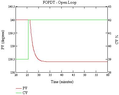
The easiest way to test this discrete time model is to execute an open loop step test that is similar to the example given in a previous tutorial (see Validating Our Heat Exchanger FOPDT Model).
Initialize:
temperature as: PV(0) = 140
controller output as: CO = 39 for n ≤ 48
Implement controller output step at time t = 25.5 min, or n = 1530:
CO = 39 for n < 1530
CO = 42 for n ≥ 1531
Simulate for 60 min, or: n = 0,1,…,3600. Display results in the plot below after 20 min (click for large view):
Controller Tuning
The formulas for calculating the PI tuning values can now be tested using the discrete time process model that was generated above.
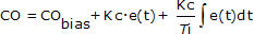
The tuning values are for the PI controller that is expressed in the continuous time or analog form as:
The PI controller tuning values are calculated using the equations provided in previous tutorials (see PI Control of the Heat Exchanger). Following that procedure, the desired closed loop time constant, Tc, must be chosen to determine how quickly or how aggressive the desired response should be.
For an aggressive response, Tc should be the larger of 0.1Tp or 0.8Өp. As listed above, Tp = 1.3 min and Өp = 0.8 min for the heat exchanger. Using these model parameters, then:
Tc = max(0.1Tp, 0.8Өp) = 0.64
A moderate Tc of the larger of 1.0Tp or 8.0Өp will produce a response with no overshoot. We will use this rule in the closed loop simulation below:
Tc = max(1.0Tp, 8.0Өp) = 6.4
Using this moderate Tc, we can now compute the controller gain, Kc, and integrator term,Ti:

Closed Loop PI Control
The function logic that follows implements the PI controller and the discrete time FOPDT model’s response. The controller uses the PV to calculate a CO that is used later by the plant model. How much later is determined by the dead time. The model then responds by changing the PV. This new PV is then used in the next iteration.
– compute controller error:
ERR = SP – PV
– compute COp, the proportional contribution to CO:
COp = Kc·ERR
– compute COi, the integral contribution to CO:
COi = COi + (Kc·T·ERR)/Ti
– compute the total controller output:
CO = COp + COi
– compute the process response at the next step n using the time-delayed CO:
PV(n+1) = A·PV(n) + B·Kp·CO(n–Өp) + C
| Aside: The integral contribution to CO can include the integrator limiting technique talked about in the Integral (Reset) Windup and Jacketing Logic post with the expression: |
We initialize the variables at time t=0 by assuming that there is no error and the system is in a quiescent state. Thus, all of the control output, CO, is due only to the integrator term, COi:
PV(0) = 140; CO(0) = 39; COi(0) = CO(0)
The plot below (click for large view) shows the response of the closed loop system over a simulation time of 60 minutes. The set point is stepped from 140 to 138.4 at time t = 25.5 minutes.
The function logic above calculates the PV and CO for each time period in the 60 minute simulation. Note that there are three CO type variables. CO is the current control value, COi is the current integrator contribution to the CO, and CO(n-Өp) is the delayed CO that simulates the dead time.
When programming the functions, additional logic is required keep from using indexes less than 0.
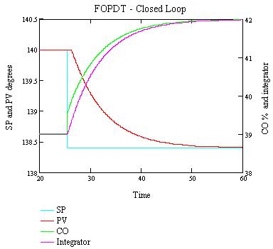
Notice that to prevent overshoot, the rate at which the controller’s integrator output, COi, responds or winds up must be limited so the total control output does not exceed the final steady state control output, and final steady state control output is not reached before the system starts to respond. The way I think about it is that the function is calculating the value for Kc so this goal can be achieved.
Also notice that with moderate tuning, the closed loop response is much slower than the open loop response.
__________
About the Author
Peter Nachtwey is the president and head engineer of Delta Computer systems which is a manufacturer of motion control and color sensor products. Peter Nachtwey has more than 20 years of experience developing hydraulic, pneumatic, electrical motion control and vision systems and products for industrial applications.
Peter Nachtwey
President
Delta Computer Systems, Inc.
11719 NE 95th St Suite D
Vancouver, WA 98682-2444
(360) 255-8688
Email: peter@deltamotion.com
Web: http://www.deltamotion.com
Addendum
Below is a Scilab program the implements the linear discrete heat exchanger simulation. The program below can be cut and pasted into Scilab’s editor.
// SIMPLE HEAT EXCHANGER CALCULATION FROM CONTROL GURU
// http://controlguru.com
// NEW SCILAB USERS SHOULD BUY
// Modeling and Simulation in Scilab/Scicos
// NOTE, EXPRESSIONS ENDING WITH SEMICOLONS WILL NOT PRINT WHEN EXECUTED
// EXPRESSIOBS WITHOUT SEMICOLONS WILL DISPLAY THE ASSIGNED VALUE(S)
Kp=-0.533; // PLANT GAIN, UNITLESS
Tp=1.3*60; // PLANT TIME CONSNTAT IN SECONDS
DT=round(0.8*60); // PLANT DEAD TIME IN SECONDS
T=1; // UPDATE TIME IN SECONDS
PVss=140-39*Kp; // STEADY STATE TEMPERATURE
// CALCULATE THE MODEL COEFFICIENTS
A=exp(-T/Tp); // DISCRETE TIME TRANSITION MATRIX WITH ONLY ONE ELEMENT
B=Kp*(1-A); // DISCRETE TIME INPUT COUPLING MATRIX
C=(1-A)*PVss; // OFFSET OR SYSTEM BIAS SO SYSTEM GOES TO PVss WITH NO CONTROL
// CALCULATE THE PI CONTROLLER GAINS USING THE IMC METHOD AS FOUND ON CONTROLGURU
Tc=max(Tp,8*DT); // DESIRED CLOSED LOOP TIME CONSTANT
Kc=Tp/(Kp*(Tc+DT)); // CONTROLLER PROPORTIONAL GAIN
Ti=Tp; // CONTROLLER INTEGRATOR TIME CONSTANT
for n=1:3600 // SIMULATE 60 MINUTES OF TIME. n = SECONDS
// INITIAL CONDITIONS, NOTE SCILAB ARRAYS START WITH 1
if n == 1 then
SP(1)=140; // INITIAL SET POINT
PV(1)=140; // PROCESS VARIABLE, TEMPERATURE = 140
CV(1)= 39; // CONTROL VARIABLE, OUTPUT % = 39%
CVi(1)=CV(1); // THE INTEGRATOR CONTRIBUTION TO THE OUTPUT. 39%
CVp(1)=0; // PROPORTIONAL CONTRIBBUTION TO THE OUTPUT
// ASSUME INITALY THERE IS NOT ERROR
end
// GENERATE THE SP AS A FUNCTION OF TIME
// IN THIS CASE THERE IS JUST A SIMPLE STEP CHANGE AS IN THE CONTROLGURU EXAMPLE
// ADD MORE SP CHANGES BY USING THE elsif KEYWORD
if n