The derivative action of a PID controller can cause noise in the measured process variable (PV) to be amplified and reflected as “chatter” in the controller output (CO) signal. Signal filters, implemented as either analog hardware or digital software, offer a popular solution to this problem.

If noise is impacting controller performance, our first attempts should be to locate and correct the underlying fault. Filters are poor cures for a bad design or failing equipment.

If we decide to employ a filter in our loop, an algorithm designed to smooth the controller output signal holds some allure.

The CO Filter Architecture
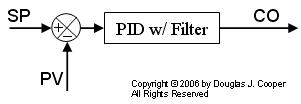
Below is a loop architecture with a PID controller followed by a controller output filter.

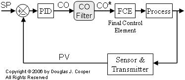
The benefits of this architecture include:

▪	A CO filter works to limit large controller output moves regardless of the underlying cause. As a result, CO filters can reduce persistent controller output fluctuations that cause wear in a mechanical final control element (FCE).
▪	A CO filter is a single solution that addresses both a noisy PV measurement problem and computational oddities that may exist in our vendor’s particular PID algorithm,
▪	Perhaps most important, the tuning recipe we have employed so successfully with PI and PID algorithms can be directly applied to a PID with CO filter architecture.

PID Plus External Filter
As shown above, the filter computation is performed after the PID controller has computed the CO. Below, the PID controller output is computed using the non-interacting, dependent, ideal form, but any of the popular algorithms can be used with this “PID plus filter” architecture:

  Where:
    CO = controller output signal (the wire out)
    CO_bias = controller bias; set by bumpless transfer
    e(t) = current controller error, defined as SP – PV
    SP = set point
    PV = measured process variable (the wire in)
    Kc = controller gain, a tuning parameter
    Ti = reset time, a tuning parameter
    Td = derivative time, a tuning parameter

The Filtering Algorithm
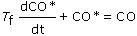
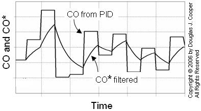
A first order filter yields a smoothed CO* value as:

  Where:
    CO = raw PID controller output signal
    CO* = filtered CO signal sent to FCE (e.g., valve)
    T_f = filter time constant, a tuning parameter

A comparison of the first order filter above to a general first order plus dead time (FOPDT) model form reveals that:

▪	The gain (or scaling factor) of the filter is one. That is, the filtered CO* has the same zero, span and units as the CO value from the PID algorithm.
▪	There is no dead time built into the filter. The CO* forwarded to the FCE is computed immediately after the PID algorithm yields the raw (unfiltered) CO signal.
▪	The degree of filtering, or how quickly CO* moves toward the unfiltered CO value, is set by Tf , the filter time constant.

Filtering Adds Delay
The degree of smoothing depends on the size of the filter time constant, T_f :

▪	A smaller Tf means CO* moves quickly and follows closer to changes in CO, so there is little filtering or smoothing of the signal.
▪	A larger Tf means CO* responds more slowly to changes in CO, so the filtering or smoothing is greater.

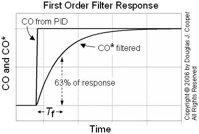
Shown below is a series of CO signals from a PID controller. Also shown is the filtered CO* trace using the same T_f as in the plot above.

As smoothing (or filter time, T_f) increases, the filtered signal may become more visually appealing, but more filtering means additional information delay in the control loop computation.

As delay increases in a control loop, the best achievable control performance decreases. The design challenge is to find the careful balance between signal smoothing and information delay to achieve the controller performance we desire for our process.

Combining Controller Plus Filter
To use our tuning recipe, we must first combine the controller and filter into a single unified equation. Since both equations above have CO isolated on one side of the equal sign, we can set the two equations equal to yield:

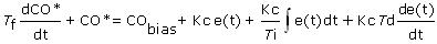
Moving the left-most term to the right-hand side produces the unified PID with Filter equation:

Unified PID With Filter Form
For design and tuning purposes going forward, we will use the unified PID with Filter equation form, as if it were represented by the schematic:

As implied by this diagram, we will drop the CO versus CO* nomenclature and simply write the unified PID with Filter equation as:

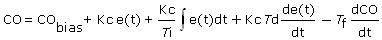
Please be aware that this is identical in every way to the PID with external filter algorithm derived earlier in this article. We recast it only so the tuning correlations are consistent in appearance and application with those of the PI and PID forms presented in earlier articles.

Filter Time Constant
Many commercial controllers that include some form of a PID with Filter algorithm cast the filter time constant as a fraction of the controller derivative time, or:

The unified PID with Filter algorithm then becomes:

We will use this aTd form in the example that follows. If your controller output filter uses T_f, the conversion is computed: T_f = aTd.

Discrete-Time Implementation
While a CO filter offers potential for benefit in loops with noise and/or delicate mechanical FCEs, if our vendor does not offer the option, we must program the filter ourselves. Fortunately, the code is straightforward.

As above, the first order filtering algorithm is expressed:

In discrete-time form, we write:

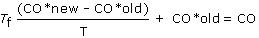
or

  CO^*new = CO^*old + (T/T_f)(CO - CO^*old)

Where T is the loop sample time and CO is the unfiltered PID signal.

In a computer program, the “new” CO* is computed directly from the “old” CO* value at each loop, so we do not need to keep track of these labels. The filter computation can be programmed in one line as:

  COstar = COstar + (T/T_f)(CO – COstar)

Applying the CO Filter
We explore an example of PID control with CO filtering applied to the heat exchanger and jacketed stirred reactor process.

Return to the Table of Contents to learn more.

Copyright © 2006 by Douglas J. Cooper. All Rights Reserved.